bootlm
 Uses bootstrap to calculate confidence intervals (and p-values) for the
 regression coefficients from a linear model and performs N-way ANOVA.

 -- Function File: bootlm (Y, X)
 -- Function File: bootlm (Y, GROUP)
 -- Function File: bootlm (Y, GROUP, ..., NAME, VALUE)
 -- Function File: bootlm (Y, GROUP, ..., 'dim', DIM)
 -- Function File: bootlm (Y, GROUP, ..., 'continuous', CONTINUOUS)
 -- Function File: bootlm (Y, GROUP, ..., 'model', MODELTYPE)
 -- Function File: bootlm (Y, GROUP, ..., 'standardize', STANDARDIZE)
 -- Function File: bootlm (Y, GROUP, ..., 'varnames', VARNAMES)
 -- Function File: bootlm (Y, GROUP, ..., 'method', METHOD)
 -- Function File: bootlm (Y, GROUP, ..., 'method', 'bayesian', 'prior', PRIOR)
 -- Function File: bootlm (Y, GROUP, ..., 'alpha', ALPHA)
 -- Function File: bootlm (Y, GROUP, ..., 'display', DISPOPT)
 -- Function File: bootlm (Y, GROUP, ..., 'contrasts', CONTRASTS)
 -- Function File: bootlm (Y, GROUP, ..., 'nboot', NBOOT)
 -- Function File: bootlm (Y, GROUP, ..., 'clustid', CLUSTID)
 -- Function File: bootlm (Y, GROUP, ..., 'blocksz', BLOCKSZ)
 -- Function File: bootlm (Y, GROUP, ..., 'posthoc', POSTHOC)
 -- Function File: bootlm (Y, GROUP, ..., 'seed', SEED)
 -- Function File: STATS = bootlm (...)
 -- Function File: [STATS, BOOTSTAT] = bootlm (...)
 -- Function File: [STATS, BOOTSTAT, AOVSTAT] = bootlm (...)
 -- Function File: [STATS, BOOTSTAT, AOVSTAT, PRED_ERR] = bootlm (...)
 -- Function File: [STATS, BOOTSTAT, AOVSTAT, PRED_ERR, MAT] = bootlm (...)
 -- Function File: 'MAT = bootlm (Y, GROUP, ..., 'nboot', 0)'

        Fits a linear model with categorical and/or continuous predictors (i.e.
     independent variables) on a continuous outcome (i.e. dependent variable)
     and computes the following statistics for each regression coefficient:
          - name: the name(s) of the regression coefficient(s)
          - coeff: the value of the regression coefficient(s)
          - CI_lower: lower bound(s) of the 95% confidence interval (CI)
          - CI_upper: upper bound(s) of the 95% confidence interval (CI)
          - p-val: two-tailed p-value(s) for the parameter(s) being equal to 0
        By default, confidence intervals and Null Hypothesis Significance Tests
     (NHSTs) for the regression coefficients (H0 = 0) are calculated by wild
     (cluster) unrestricted bootstrap-t and are robust when normality and
     homoscedasticity cannot be assumed [1].

        Usage of this function is very similar to that of 'anovan'. Data (Y)
     is a numeric variable, and the predictor(s) are specified in GROUP (a.k.a.
     X), which can be a vector, matrix, or cell array. For a single predictor,
     GROUP can be a vector of numbers, logical values or characters, or a cell
     array of numbers, logical values or character strings, with the same
     number of elements (n) as Y. For K predictors, GROUP can be either a
     1-by-K, where each column corresponds to a predictor as defined above,
     an n-by-K cell array, or an n-by-K array of numbers or characters. If
     Y, or the definitions of each predictor in GROUP, are not column vectors,
     then they will be transposed or reshaped to be column vectors. Rows of
     data whose outcome (Y) or value of any predictor is NaN or Inf are
     excluded. For examples of function usage, please see demonstrations in
     the manual at:

     https://gnu-octave.github.io/statistics-resampling/function/bootlm.html

     Note that if GROUP is defined as a design matrix X, containing (one or
     more) continuous predictors only, a constant term (intercept) should
     not be included in X - one is automatically added to the model. For models
     containing any categorical predictors, the 'bootlm' function creates the
     design matrix for you. If you have already constructed a design matrix,
     consider using the functions 'bootwild' and 'bootbayes' instead.

     'bootlm' can take a number of optional parameters as name-value
     pairs.

     '[...] = bootlm (Y, GROUP, ..., 'varnames', VARNAMES)'

       <> VARNAMES must be a cell array of strings with each element
          containing a predictor name for each column of GROUP. By default
          (if not parsed as optional argument), VARNAMES are
          'X1','X2','X3', etc.

     '[...] = bootlm (Y, GROUP, ..., 'continuous', CONTINUOUS)'

       <> CONTINUOUS is a vector of indices indicating which of the
          columns (i.e. predictors) in GROUP should be treated as
          continuous predictors rather than as categorical predictors.
          The relationship between continuous predictors and the outcome
          should be linear.

     '[...] = bootlm (Y, GROUP, ..., 'model', MODELTYPE)'

       <> MODELTYPE can specified as one of the following:

             o 'linear' (default): compute N main effects with no
               interactions.

             o 'interaction': compute N effects and N*(N-1) interactions

             o 'full': compute the N main effects and interactions at
               all levels

             o a scalar integer: representing the maximum interaction
               order

             o a matrix of term definitions: each row is a term and
               each column is a predictor

               -- Example:
               A two-way design with interaction would be: [1 0; 0 1; 1 1]

     '[...] = bootlm (Y, GROUP, ..., 'standardize', STANDARDIZE)'

       <> STANDARDIZE can be either 'off' (or false, default) or 'on' (or true),
          which controls whether the outcome and any continuous predictors in
          the model should be converted to standard scores) before model
          fitting to give standardized regression coefficients. Please see the
          documentation relating to the 'posthoc' input argument to read about
          further consequences of turning on 'standardize'.

     '[...] = bootlm (Y, GROUP, ..., 'method', METHOD)'

       <> METHOD can be specified as one of the following:

             o 'wild' (default): Wild bootstrap-t, using the 'bootwild'
               function. Please see the help documentation below and in the
               function 'bootwild' for more information about this method [1].

             o 'bayesian': Bayesian bootstrap, using the 'bootbayes' function.
                Please see the help documentation below and in the function
               'bootbayes' for more information about this method [2]. This
                method is well-optimized for large data sets.

             Note that p-values are a frequentist concept and are only computed
             and returned from bootlm when the METHOD is 'wild'. Since the wild
             bootstrap method here (based on Webb's 6-point distribution)
             imposes symmetry on the sampling of the residuals, we recommend
             using 'wild' bootstrap for (two-sided) hypothesis tests, and
             instead use 'bayesian' bootstrap with the 'auto' prior setting
             (see below) for estimation of precision/uncertainty (e.g. credible
             intervals).

     '[...] = bootlm (Y, GROUP, ..., 'method', 'bayesian', 'prior', PRIOR)'

       <> Sets the prior for Bayesian bootstrap. Possible values are:

             o scalar: A non-negative (>= 0) scalar that parametrizes the
                  symmetric Dirichlet used to generate weights for linear
                  least squares and the nonparametric Bayesian bootstrap
                  posterior.

             o 'auto' (default): Sets value(s) for PRIOR that effectively
                  incorporates Bessel's correction a priori such that the
                  variance of the posterior (i.e. of the rows of BOOTSTAT)
                  becomes an unbiased estimator of the sampling variance*.
                  The bootlm function uses a dedicated prior for each linear
                  estimate. Please see the help documentation for the function
                  'bootbayes' for more information about the prior [2].

     '[...] = bootlm (Y, GROUP, ..., 'method', 'bayesian', 'prior', PRIOR)'

       <> Sets the prior for Bayesian bootstrap. Possible values are:

             o scalar: A non-negative (>= 0) scalar (Dirichlet concentration
                 alpha) that parametrizes the symmetric Dirichlet used to
                 generate weights for linear least squares and the
                 nonparametric Bayesian bootstrap posterior. (Note: alpha = 0
                 is the Haldane case.)

             o 'auto' (default): Applies a degrees-of-freedom style correction
                 so that the posterior variance (rows of BOOTSTAT) becomes an
                 unbiased estimator of sampling variance. bootlm uses a
                 dedicated prior for each linear estimate*. See 'bootbayes'
                 for the exact formulas and details [2].

     '[...] = bootlm (Y, GROUP, ..., 'alpha', ALPHA)'

       <> ALPHA is numeric and sets the lower and upper bounds of the
          confidence or credible interval(s). The value(s) of ALPHA must be
          between 0 and 1. ALPHA can either be:

             o scalar: Set the central mass of the intervals to 100*(1-ALPHA)%.
                  For example, 0.05 for a 95% interval. If METHOD is 'wild',
                  then the intervals are symmetric bootstrap-t confidence
                  intervals [1]. If METHOD is 'bayesian', then the intervals
                  are shortest probability credible intervals [2].

             o vector: A pair of probabilities defining the lower and upper
                  and upper bounds of the interval(s) as 100*(ALPHA(1))% and
                  100*(ALPHA(2))% respectively. For example, [.025, .975] for
                  a 95% interval. If METHOD is 'wild', then the intervals are
                  asymmetric bootstrap-t confidence intervals [1]. If METHOD is
                  'bayesian', then the intervals are simple percentile credible
                  intervals [2].

               The default value of ALPHA is the scalar: 0.05.

     '[...] = bootlm (Y, GROUP, ..., 'display', DISPOPT)'

       <> DISPOPT can be either 'on' (or true, default) or 'off' (or false)
          and controls the display of the model formula, a table of model
          parameter estimates and a figure of diagnostic plots. The p-values
          are formatted in APA-style.

     '[...] = bootlm (Y, GROUP, ..., 'contrasts', CONTRASTS)'

       <> CONTRASTS can be specified as one of the following:

             o A string corresponding to one of the built-in contrasts
               listed below:

                  o 'treatment' (default): Treatment contrast (or dummy)
                    coding. The intercept represents the mean of the first
                    level of all the predictors. Each slope coefficient
                    compares one level of a predictor (or interaction
                    between predictors) with the first level for that/those
                    predictor(s), at the first level of all the other
                    predictors. The first (or reference level) of the
                    predictor(s) is defined as the first level of the
                    predictor (or combination of the predictors) listed in
                    the GROUP argument. This type of contrast is ideal for
                    one-way designs or factorial designs of nominal predictor
                    variables that have an obvious reference or control group.

                  o 'anova' or 'simple': Simple (ANOVA) contrast coding. The
                    intercept represents the grand mean. Each slope coefficient
                    represents the difference between one level of a predictor
                    (or interaction between predictors) to the first level for
                    that/those predictor(s), averaged over all levels of the
                    other predictor(s). The first (or reference level) of the
                    predictor(s) is defined as the first level of the predictor
                    (or combination of the predictors) listed in the GROUP
                    argument. The columns of this contrast coding scheme sum
                    to zero. This type of contrast is ideal for nominal
                    predictor variables that have an obvious reference or
                    control group and that are modelled together with a
                    covariate or blocking factor.

                  o 'poly': Polynomial contrast coding for trend analysis.
                    The intercept represents the grand mean. The remaining
                    slope coefficients returned are for linear, quadratic,
                    cubic etc. trends across the levels. In addition to the
                    columns of this contrast coding scheme summing to zero,
                    this contrast coding is orthogonal (i.e. the off-diagonal
                    elements of its autocovariance matrix are zero) and so
                    the slope coefficients are independent. This type of
                    contrast is ideal for ordinal predictor variables, in
                    particular, predictors with ordered levels that are evenly
                    spaced.

                  o 'helmert': Helmert contrast coding. The intercept
                    represents the grand mean. Each slope coefficient
                    represents the difference between one level of a predictor
                    (or interaction between predictors) with the mean of the
                    subsequent levels, where the order of the predictor levels
                    is as they appear in the GROUP argument. In addition to the
                    columns of this contrast coding scheme summing to zero,
                    this contrast coding is orthogonal (i.e. the off-diagonal
                    elements of its autocovariance matrix are zero) and so the
                    slope coefficients are independent. This type of contrast
                    is ideal for predictor variables that are either ordinal,
                    or nominal with their levels ordered such that the contrast
                    coding reflects tests of some hypotheses of interest about
                    the nested grouping of the predictor levels. Note that the
                    the one-level predictor is the reference and is subtracted
                    from from the mean of the subsequent predictor levels.

                  o 'effect': Deviation effect coding. The intercept represents
                    the grand mean. Each slope coefficient compares one level
                    of a predictor (or interaction between predictors) with the
                    grand mean. Note that a slope coefficient is omitted for
                    the first level of the predictor(s) listed in the GROUP
                    argument. The columns of this contrast coding scheme sum to
                    zero. This type of contrast is ideal for nominal predictor
                    variables when there is no obvious reference group.

                  o 'sdif' or 'sdiff': Successive differences contrast coding.
                    The intercept represents the grand mean. Each slope
                    coefficient represents the difference between one level of
                    a predictor (or interaction between predictors) to the
                    previous one, where the order of the predictor levels is
                    as they appear in the GROUP argument. The columns of this
                    contrast coding coding scheme sum to zero. This type of
                    contrast is ideal for ordinal predictor variables.

            <> A matrix containing a custom contrast coding scheme (i.e.
               the generalized inverse of contrast weights). Rows in
               the contrast matrices correspond to predictor levels in the
               order that they first appear in the GROUP column. The
               matrix must contain the same number of columns as there
               are the number of predictor levels minus one.

          If the linear model contains more than one predictor and a
          built-in contrast coding scheme was specified, then those
          contrasts are applied to all predictors. To specify different
          contrasts for different predictors in the model, CONTRASTS should
          be a cell array with the same number of cells as there are
          columns in GROUP. Each cell should define contrasts for the
          respective column in GROUP by one of the methods described
          above. If cells are left empty, then the default contrasts
          are applied. Contrasts for cells corresponding to continuous
          predictors are ignored.

     '[...] = bootlm (Y, GROUP, ..., 'nboot', NBOOT)'

       <> Specifies the number of bootstrap resamples, where NBOOT must be a
          positive integer. If empty, the default value of NBOOT is 9999.

     '[...] = bootlm (Y, GROUP, ..., 'clustid', CLUSTID)'

       <> Specifies a vector or cell array of numbers or strings respectively
          to be used as cluster labels or identifiers. Rows of the data with
          the same CLUSTID value are treated as clusters with dependent errors.
          If CLUSTID is a row vector or a two dimensional array or matrix, then
          it will be transposed or reshaped to be a column vectors. If empty
          (default), no clustered resampling is performed and all errors are
          treated as independent. The standard errors computed are cluster-
          robust standard errors.

     '[...] = bootlm (Y, GROUP, ..., 'blocksz', BLOCKSZ)'

       <> Specifies a scalar, which sets the block size for bootstrapping when
          the errors have serial dependence. Rows of the data within the same
          block are treated as having dependent errors. If empty (default),
          no clustered resampling is performed and all errors are treated
          as independent. The standard errors computed are cluster robust.

     '[...] = bootlm (Y, GROUP, ..., 'dim', DIM)'

       <> DIM can be specified as one of the following:

             o a cell array of strings corresponding to variable names defined
               VARNAMES, or

             o a scalar or vector specifying the dimension(s),

          over which 'bootlm' calculates and returns estimated marginal means
          instead of regression coefficients. For example, the value [1 3]
          computes the estimated marginal mean for each combination of the
          levels of the first and third predictors. The rows of the estimates
          returned are sorted according to the order of the dimensions
          specified in DIM. The default value of DIM is empty, which makes
          'bootlm' return the statistics for the model coefficients. If DIM
          is, or includes, a continuous predictor then 'bootlm' will return an
          error. The following statistics are printed when specifying 'dim':
             - name: the name(s) of the estimated marginal mean(s)
             - mean: the estimated marginal mean(s)
             - CI_lower: lower bound(s) of the 95% confidence interval (CI)
             - CI_upper: upper bound(s) of the 95% confidence interval (CI)
             - N: the number of independent sampling units used to compute CIs

     '[...] = bootlm (Y, GROUP, ..., 'posthoc', POSTHOC)'

       <> When DIM is specified, POSTHOC comparisons along DIM can be one of
          the following:

             o empty or 'none' (default) : No posthoc comparisons are performed.
               The statistics returned are for the estimated marginal means.

             o 'pairwise' : Pairwise comparisons are performed.

             o 'trt_vs_ctrl' : Treatment vs. Control comparisons are performed.
               Control corresponds to the level(s) of the predictor(s) listed
               within the first row of STATS when POSTHOC is set to 'none'.

             o {'trt_vs_ctrl', k} : Treatment vs. Control comparisons are
               performed. The control is group number k as returned when
               POSTHOC is set to 'none'.

             o a two-column numeric matrix defining each pair of comparisons,
               where each number in the matrix corresponds to the row number
               of the estimated-marginal means as listed for the same value(s)
               of DIM and when POSTHOC is set to 'none'. The comparison
               corresponds to the row-wise differences: column 1 - column 2.
               See demo 6 for an example.

          All of the posthoc comparisons use the step-down max |T| procedure
          to control the type I error rate, but the confidence intervals are
          not adjusted for multiple comparisons [3]. If the 'standardize' input
          argument set to 'on', the estimates, confidence intervals and
          bootstrap statistics for the comparisons are converted to estimates
          of Cohen's d standardized effect sizes. Cohen's d here is calculated
          from the residual standard deviation, which is estimated from the
          standard errors and the sample sizes. As such, the effect sizes
          calculated exclude variability attributed to other predictors in
          the model.

     '[...] = bootlm (Y, GROUP, ..., 'seed', SEED)' initialises the Mersenne
     Twister random number generator using an integer SEED value so that
     'bootlm' results are reproducible.

     'bootlm' can return up to four output arguments:

     'STATS = bootlm (...)' returns a structure with the following fields:
       - 'method': The bootstrap method
       - 'name': The names of each of the estimates
       - 'estimate': The value of the estimates
       - 'CI_lower': The lower bound(s) of the confidence/credible interval(s)
       - 'CI_upper': The upper bound(s) of the confidence/credible interval(s)
       - 'pval': The p-value(s) for the hypothesis that the estimate(s) == 0
       - 'fpr': The minimum false positive risk (FPR) for each p-value [4].
       - 'N': The number of independent sampling units used to compute CIs
       - 'prior': The prior used for Bayesian bootstrap. This will return a
                  scalar for regression coefficients, or a P x 1 or P x 2
                  matrix for estimated marginal means or posthoc tests
                  respectively, where P is the number of parameter estimates.
       - 'levels': A cell array with the levels of each predictor.
       - 'contrasts': A cell array of contrasts associated with each predictor.

          Note that the p-values returned are truncated at the resolution
          limit determined by the number of bootstrap replicates, specifically
          1 / (NBOOT + 1). Values for the minumum false positive risk are
          computed using the Sellke-Berger approach. The following fields are
          only returned when 'estimate' corresponds to model regression
          coefficients: 'levels' and 'contrasts'.

     '[STATS, BOOTSTAT] = bootlm (...)' also returns a P x NBOOT matrix of
     bootstrap statistics for the estimated parameters, where P is the number
     of parameters estimated in the model. Depending on the DIM and POSTHOC
     input arguments set by the user, the estimated parameters whose bootstrap
     statistics are returned will be either regression coefficients, the
     estimated marginal means, or the mean differences between groups of a
     categorical predictor for posthoc testing.

     '[STATS, BOOTSTAT, AOVSTAT] = bootlm (...)' also computes bootstrapped
     ANOVA statistics* and returns them in a structure with the following
     fields:
       - 'MODEL': The formula of the linear model(s) in Wilkinson's notation
       - 'SS': Sum-of-squares
       - 'DF': Degrees of freedom
       - 'MS': Mean-squares
       - 'F': F-Statistic
       - 'PVAL': p-values
       - 'FPR': The minimum false positive risk for each p-value [3]
       - 'SSE': Sum-of-Squared Error
       - 'DFE': Degrees of Freedom for Error
       - 'MSE': Mean Squared Error

       The ANOVA implemented uses sequential (type I) sums-of-squares and so
       the results and their interpretation depend on the order** of predictors
       in the GROUP variable (when the design is not balanced). Thus, the null
       model used for comparison for each model is the model listed directly
       above it in AOVSTAT; for the first model, the null model is the
       intercept-only model. The procedure here for bootstrapping ANOVA is
       performed with the null hypothesis imposed and requires that the method
       used is 'wild' bootstrap AND that no other statistics are requested
       (i.e. estimated marginal means or posthoc tests).

       The bootlm function treats all model predictors as fixed effects during
       ANOVA tests. Note also that the bootlm function can be used to compute
       p-values for ANOVA with accounting for dependence structures such as
       block or nested designs by wild cluster bootstrap resampling (see the
!      'clustid' or 'blocksz' option).

       ** See demo 7 for an example of how to obtain results for ANOVA using
          type II sums-of-squares, which test hypotheses that give results
          invariant to the order of the predictors, regardless of whether
          sample sizes are equal or not.

     '[STATS, BOOTSTAT, AOVSTAT, PRED_ERR] = bootlm (...)' also computes
     refined bootstrap estimates of prediction error* and returns statistics
     derived from it in a structure containing the following fields:
       - 'MODEL': The formula of the linear model(s) in Wilkinson's notation
       - 'PE': Bootstrap estimate of prediction error [5]
       - 'PRESS': Bootstrap estimate of predicted residual error sum of squares
       - 'RSQ_pred': Bootstrap estimate of predicted R-squared
       - 'EIC': Extended (Efron) Information Criterion [6]
       - 'RL': Relative likelihood (compared to the intercept-only model)
       - 'Wt': EIC expressed as weights

       The linear models evaluated are the same as for AOVSTAT, except that the
       output also includes the statistics for the intercept-only model. Note
       that PRED_ERR statistics are only returned when the method used is
       'wild' bootstrap AND when no other statistics are requested (i.e.
       estimated marginal means or posthoc tests). Computations of the
       statistics in PRED_ERR are compatible with the 'clustid' and 'blocksz'
        options. Note that it is possible (and not unusual) to get a negative
       value for RSQ-pred, particularly for the intercept-only model.

     * If the parallel computing toolbox (Matlab) or package (Octave) is
       installed and loaded, then these computations will be automatically
       accelerated by parallel processing on platforms with multiple processors.

     '[STATS, BOOTSTAT, AOVSTAT, PRED_ERR, MAT] = bootlm (...)' also returns
     a structure containing the design matrix of the predictors (X), the raw
     regression coefficients (b), the outcome (Y), the column vector (ID) of
     arbitrary numeric identifiers for the independent sampling units, the
     cell array of contrast/coding matrices (C) used to generate X, and the
     hypothesis matrix (L) for computing any specified estimated marginal means
     or posthoc comparisons.

     'MAT = bootlm (Y, GROUP, ..., 'nboot', 0)'

       <> Performs the least-squares fit only and returns MAT without any
          bootstrap resampling. All other input options are accepted (even if
          some are ignored), but only one output argument can be requested.
          The 'display' option, if true creates the figure or diagnostic plots
          but does not print any results to stdout.

  Bibliography:
  [1] Penn, A.C. statistics-resampling manual: `bootwild` function reference.
        https://gnu-octave.github.io/statistics-resampling/function/bootwild.html
        and references therein. Last accessed 02 Sept 2024.
  [2] Penn, A.C. statistics-resampling manual: `bootbayes` function reference.
        https://gnu-octave.github.io/statistics-resampling/function/bootbayes.html
        and references therein. Last accessed 02 Sept 2024.
  [3] Westfall, P. H., & Young, S. S. (1993). Resampling-Based Multiple
        Testing: Examples and Methods for p-Value Adjustment. Wiley.
  [4] David Colquhoun (2019) The False Positive Risk: A Proposal Concerning
        What to Do About p-Values, The American Statistician, 73:sup1, 192-201
  [5] Efron and Tibshirani (1993) An Introduction to the Bootstrap.
        New York, NY: Chapman & Hall. pg 247-252
  [6] Konishi & Kitagawa (2008), "Bootstrap Information Criterion" In:
        Information Criteria and Statistical Modeling. Springer Series in
        Statistics. Springer, NY.

  bootlm (version 2026.07.06)
  Author: Andrew Charles Penn
  https://www.researchgate.net/profile/Andrew_Penn/

  Copyright 2019 Andrew Charles Penn
  This program is free software: you can redistribute it and/or modify
  it under the terms of the GNU General Public License as published by
  the Free Software Foundation, either version 3 of the License, or
  (at your option) any later version.

  This program is distributed in the hope that it will be useful,
  but WITHOUT ANY WARRANTY; without even the implied warranty of
  MERCHANTABILITY or FITNESS FOR A PARTICULAR PURPOSE. See the
  GNU General Public License for more details.

  You should have received a copy of the GNU General Public License
  along with this program.  If not, see http://www.gnu.org/licenses/
Demonstration 1
The following code
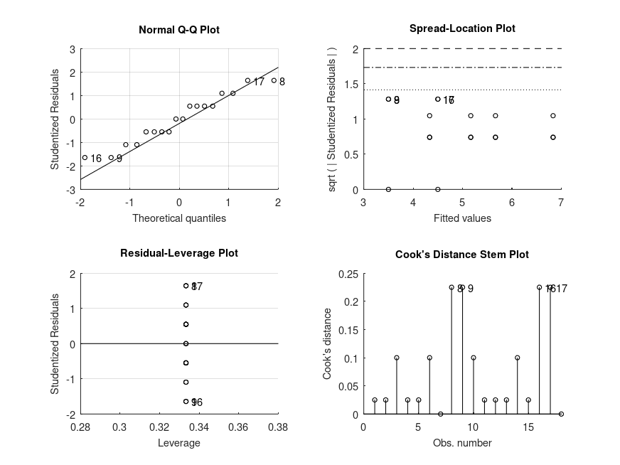
 % Two-sample unpaired test on independent samples (equivalent to Welch's
 % t-test).

 score = [54 23 45 54 45 43 34 65 77 46 65]';
 gender = {'male' 'male' 'male' 'male' 'male' 'female' 'female' 'female' ...
           'female' 'female' 'female'}';

 % 95% confidence intervals and p-values for the difference in mean score
 % between males and females (computed by wild bootstrap)
 STATS = bootlm (score, gender, 'display', 'on', 'varnames', 'gender', ...
                 'dim', 1, 'posthoc','trt_vs_ctrl');

 % Standardized effect size (Cohen's d) with 95% confidence intervals and
 % total sample size for the difference in mean score between males and
 % females (computed by wild bootstrap)
 STATS = bootlm (score, gender, 'display', 'on', 'varnames', 'gender', ...
                 'dim', 1, 'posthoc','trt_vs_ctrl', 'standardize', true, ...
                 'method', 'wild');

 fprintf ('Cohen''s d [95%% CI] = %.2f [%.2f, %.2f] (N = %u)\n\n', ...
          STATS.estimate, STATS.CI_lower, STATS.CI_upper, STATS.N)

 % Standardized effect size (Cohen's d) with 95% credible intervals and
 % total sample size for the difference in mean score between males and
 % females (computed by bayesian bootstrap)
 STATS = bootlm (score, gender, 'display', 'on', 'varnames', 'gender', ...
                 'dim', 1, 'posthoc','trt_vs_ctrl', 'standardize', true, ...
                 'method', 'bayesian', 'prior', 'auto');

 fprintf ('Cohen''s d [95%% CI] = %.2f [%.2f, %.2f] (N = %u)\n\n', ...
          STATS.estimate, STATS.CI_lower, STATS.CI_upper, STATS.N)

 % 95% credible intervals for the estimated marginal means of the scores by
 % males and females (computed by Bayesian bootstrap)
 STATS = bootlm (score, gender, 'display', 'on', 'varnames', 'gender', ...
                 'dim', 1, 'method', 'bayesian', 'prior', 'auto');
Produces the following output
MODEL FORMULA (based on Wilkinson's notation):

score ~ 1 + gender

MODEL POSTHOC COMPARISONS

name                                   mean        CI_lower    CI_upper    p-adj
--------------------------------------------------------------------------------
female - male                          +10.80      -8.779      +30.38       .239


MODEL FORMULA (based on Wilkinson's notation):

score ~ 1 + gender

MODEL POSTHOC COMPARISONS

name                                   mean        CI_lower    CI_upper    p-adj
--------------------------------------------------------------------------------
female - male                          +0.7471     -0.6022     +2.096       .243

Cohen's d [95% CI] = 0.75 [-0.60, 2.10] (N = 11)


MODEL FORMULA (based on Wilkinson's notation):

score ~ 1 + gender

MODEL POSTHOC COMPARISONS

name                                   mean        CI_lower    CI_upper
--------------------------------------------------------------------------------
female - male                          +0.7500     -0.3708     +1.962

Cohen's d [95% CI] = 0.75 [-0.37, 1.96] (N = 11)


MODEL FORMULA (based on Wilkinson's notation):

score ~ 1 + gender

MODEL ESTIMATED MARGINAL MEANS

name                                   mean        CI_lower    CI_upper        N
--------------------------------------------------------------------------------
male                                   +44.20      +32.47      +53.12          5
female                                 +55.00      +42.03      +67.49          6
and the following figure
| Figure 1 |
|---|
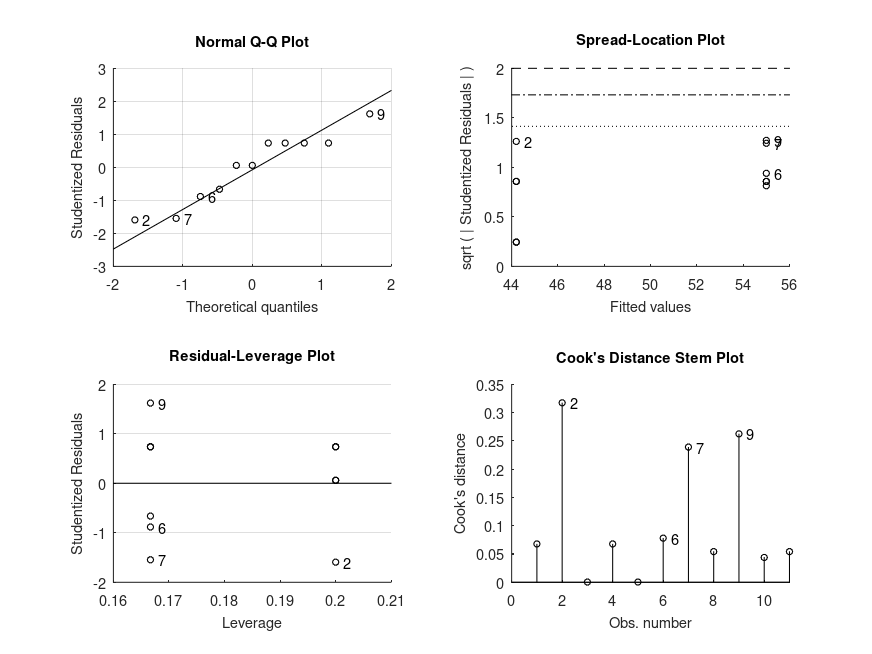 |
Demonstration 2
The following code
 % Two-sample paired test on dependent or matched samples equivalent to a
 % paired t-test using wild cluster bootstrap resampling.
 %
 % The outcome was measured before and after an intervention in different
 % subjects labelled with a unique numeric identifier.

 outcome = [59.40 46.40 46.00 49.00 32.50 45.20 60.30 54.30 45.40 38.90 ...
            64.50 52.40 49.70 48.70 37.40 49.50 59.90 54.10 49.60 48.50];
 time    = {'before' 'before' 'before' 'before' 'before' 'before' 'before' ...
            'before' 'before' 'before' 'after' 'after' 'after' 'after' ...
            'after' 'after' 'after' 'after' 'after' 'after'};
 id      = [1 2 3 4 5 6 7 8 9 10 1 2 3 4 5 6 7 8 9 10];

 % 95% confidence intervals and p-values for the difference in mean score
 % before and after treatment (computed by wild cluster bootstrap)
 STATS = bootlm (outcome, {time}, 'display', 'on', 'varnames', 'time', ...
                 'clustid', id, 'dim', 1, 'posthoc','trt_vs_ctrl');

 % 95% credible intervals for the estimated marginal means of the scores
 % before and after treatment (computed by Bayesian cluster bootstrap)
 STATS = bootlm (outcome, {time}, 'varnames', 'time', ...
                            'model', 'linear', 'display', 'on', ...
                            'dim', 1, 'method','bayesian', 'prior', 'auto');
Produces the following output
MODEL FORMULA (based on Wilkinson's notation):

outcome ~ 1 + time

MODEL POSTHOC COMPARISONS

name                                   mean        CI_lower    CI_upper    p-adj
--------------------------------------------------------------------------------
after - before                         +3.690      +1.351      +6.029       .003


MODEL FORMULA (based on Wilkinson's notation):

outcome ~ 1 + time

MODEL ESTIMATED MARGINAL MEANS

name                                   mean        CI_lower    CI_upper        N
--------------------------------------------------------------------------------
before                                 +47.74      +42.31      +53.05         10
after                                  +51.43      +46.83      +56.11         10
and the following figure
| Figure 1 |
|---|
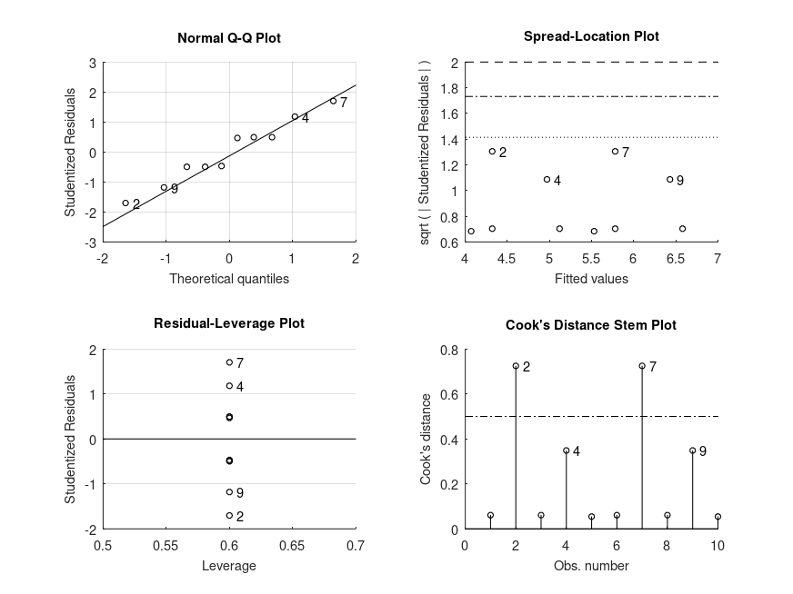 |
Demonstration 3
The following code
 % One-way design. The data is from a study on the strength of structural
 % beams, in Hogg and Ledolter (1987) Engineering Statistics. NY: MacMillan

 strength = [82 86 79 83 84 85 86 87 74 82 ...
            78 75 76 77 79 79 77 78 82 79]';
 alloy = {'st','st','st','st','st','st','st','st', ...
          'al1','al1','al1','al1','al1','al1', ...
          'al2','al2','al2','al2','al2','al2'}';

 % One-way ANOVA statistics
 [STATS, BOOTSTAT, AOVSTAT] = bootlm (strength, alloy, 'display', 'off',
                                      'varnames', 'alloy');
 fprintf ('ONE-WAY ANOVA SUMMARY\n')
 fprintf ('F = %.2f, p = %.3g for the model: %s\n', ...
          AOVSTAT.F, AOVSTAT.PVAL, AOVSTAT.MODEL{1});

 % 95% confidence intervals and p-values for the differences in mean strength
 % of the three alloys (computed by wild bootstrap)
 STATS = bootlm (strength, alloy, 'display', 'on', 'varnames', 'alloy',
                                  'dim', 1, 'posthoc','pairwise', ...
                                  'alpha', [.025, .975]);

 % 95% credible intervals for the estimated marginal means of the strengths
 % of each of the alloys (computed by Bayesian bootstrap)
 STATS = bootlm (strength, alloy, 'display', 'on', 'varnames', 'alloy', ...
                 'dim', 1, 'method','bayesian', 'prior', 'auto');
Produces the following output
ONE-WAY ANOVA SUMMARY
F = 15.40, p = 0.0005 for the model: strength ~ 1 + alloy

MODEL FORMULA (based on Wilkinson's notation):

strength ~ 1 + alloy

MODEL POSTHOC COMPARISONS

name                                   mean        CI_lower    CI_upper    p-adj
--------------------------------------------------------------------------------
st - al1                               +7.000      +3.868      +10.20      <.001
st - al2                               +5.000      +2.552      +7.498      <.001
al1 - al2                              -2.000      -4.956      +0.8968      .177


MODEL FORMULA (based on Wilkinson's notation):

strength ~ 1 + alloy

MODEL ESTIMATED MARGINAL MEANS

name                                   mean        CI_lower    CI_upper        N
--------------------------------------------------------------------------------
st                                     +84.00      +82.21      +85.73          8
al1                                    +77.00      +74.96      +79.42          6
al2                                    +79.00      +77.69      +80.47          6
and the following figure
| Figure 1 |
|---|
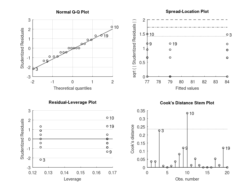 |
Demonstration 4
The following code
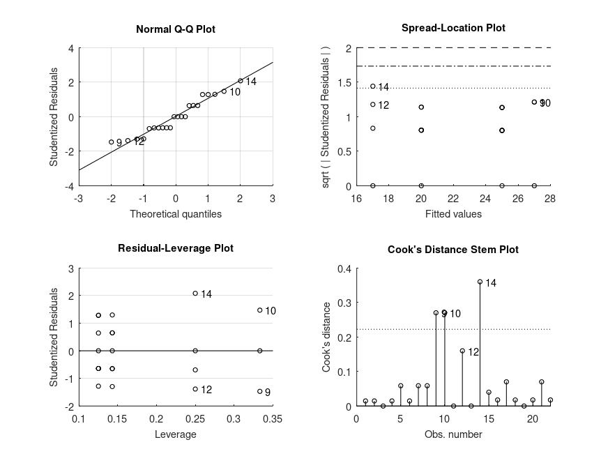
 % One-way repeated measures design analysed using wild cluster bootstrap.
 % The data is from a study on the number of words recalled by 10 subjects
 % for three time condtions, in Loftus & Masson (1994) Psychon Bull Rev.
 % 1(4):476-490, Table 2.

 words = [10 13 13; 6 8 8; 11 14 14; 22 23 25; 16 18 20; ...
          15 17 17; 1 1 4; 12 15 17;  9 12 12;  8 9 12];
 seconds = [1 2 5; 1 2 5; 1 2 5; 1 2 5; 1 2 5; ...
            1 2 5; 1 2 5; 1 2 5; 1 2 5; 1 2 5];
 subject = [ 1  1  1;  2  2  2;  3  3  3;  4  4  4;  5  5  5; ...
             6  6  6;  7  7  7;  8  8  8;  9  9  9; 10 10 10];

 % One-way ANOVA table after wild cluster bootstrap
 [STATS, BOOTSTAT, AOVSTAT] = bootlm (words, {seconds}, 'display', 'on', ...
                                   'varnames', 'seconds', 'clustid', subject);

 fprintf ('ANOVA SUMMARY\n')
 fprintf ('F = %.2f, p = %.3g for the model: %s\n', ...
          AOVSTAT.F(1), AOVSTAT.PVAL(1), AOVSTAT.MODEL{1});

 % 95% confidence intervals and p-values for the differences in mean number
 % of words recalled for the different times (using wild cluster bootstrap).
 STATS = bootlm (words, {seconds}, 'display', 'on', 'varnames', 'seconds', ...
                            'clustid', subject, 'dim', 1, ...
                            'posthoc', 'pairwise', 'alpha', [.025, .975]);

 % 95% credible intervals for the estimated marginal means of the number of
 % words recalled for each time (computed using Bayesian cluster bootstrap).
 STATS = bootlm (words, {seconds}, 'display', 'on', 'varnames', 'seconds', ...
                            'dim', 1, 'method', 'bayesian', 'prior', 'auto');
Produces the following output
MODEL FORMULA (based on Wilkinson's notation):

words ~ 1 + seconds

MODEL COEFFICIENTS

name                                   coeff       CI_lower    CI_upper    p-val
--------------------------------------------------------------------------------
(Intercept)                            +11.00      +6.994      +15.01      <.001
seconds_1                              +2.000      +1.244      +2.756      <.001
seconds_2                              +3.200      +2.521      +3.879      <.001

ANOVA SUMMARY
F = 0.74, p = 0.0021 for the model: words ~ 1 + seconds

MODEL FORMULA (based on Wilkinson's notation):

words ~ 1 + seconds

MODEL POSTHOC COMPARISONS

name                                   mean        CI_lower    CI_upper    p-adj
--------------------------------------------------------------------------------
1 - 2                                  -2.000      -2.750      -1.254       .001
1 - 5                                  -3.200      -3.855      -2.526      <.001
2 - 5                                  -1.200      -2.155      -0.2416      .020


MODEL FORMULA (based on Wilkinson's notation):

words ~ 1 + seconds

MODEL ESTIMATED MARGINAL MEANS

name                                   mean        CI_lower    CI_upper        N
--------------------------------------------------------------------------------
1                                      +11.00      +7.343      +14.59         10
2                                      +13.00      +9.173      +16.81         10
5                                      +14.20      +10.44      +17.87         10
and the following figure
| Figure 1 |
|---|
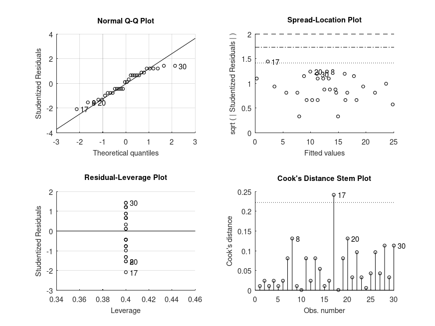 |
Demonstration 5
The following code
 % Balanced two-way design. The data is yield of cups of popped popcorn from
 % different popcorn brands and popper types, in Hogg and Ledolter (1987)
 % Engineering Statistics. NY: MacMillan

 popcorn = [5.5, 4.5, 3.5; 5.5, 4.5, 4.0; 6.0, 4.0, 3.0; ...
            6.5, 5.0, 4.0; 7.0, 5.5, 5.0; 7.0, 5.0, 4.5];
 brands = {'Gourmet', 'National', 'Generic'; ...
           'Gourmet', 'National', 'Generic'; ...
           'Gourmet', 'National', 'Generic'; ...
           'Gourmet', 'National', 'Generic'; ...
           'Gourmet', 'National', 'Generic'; ...
           'Gourmet', 'National', 'Generic'};
 popper = {'oil', 'oil', 'oil'; 'oil', 'oil', 'oil'; 'oil', 'oil', 'oil'; ...
           'air', 'air', 'air'; 'air', 'air', 'air'; 'air', 'air', 'air'};

 % Check regression coefficients corresponding to brand x popper interaction
 STATS = bootlm (popcorn, {brands, popper}, ...
                            'display', 'on', 'model', 'full', ...
                            'varnames', {'brands', 'popper'});

 % 95% confidence intervals and p-values for the differences in mean yield of
 % different popcorn brands (computed by wild bootstrap).
 STATS = bootlm (popcorn, {brands, popper}, ...
                            'display', 'on', 'model', 'full', ...
                            'varnames', {'brands', 'popper'}, ...
                            'dim', 1, 'posthoc', 'pairwise');

 % 95% credible intervals for the estimated marginal means of the yield for
 % each popcorn brand (computed by Bayesian bootstrap).
 STATS = bootlm (popcorn, {brands, popper}, ...
                            'display', 'on', 'model', 'full', ...
                            'varnames', {'brands', 'popper'}, ...
                            'dim', 1, 'method', 'bayesian', 'prior', 'auto');

 % 95% confidence intervals and p-values for the differences in mean yield
 % for different popper types (computed by wild bootstrap).
 STATS = bootlm (popcorn, {brands, popper}, ...
                            'display', 'on', 'model', 'full', ...
                            'varnames', {'brands', 'popper'}, ...
                            'dim', 2, 'posthoc', 'pairwise');

 % 95% credible intervals for the estimated marginal means of the yield for
 % each popper type (computed by Bayesian bootstrap).
 STATS = bootlm (popcorn, {brands, popper}, ...
                            'display', 'on', 'model', 'full', ...
                            'varnames', {'brands', 'popper'}, ...
                            'dim', 2, 'method', 'bayesian', 'prior', 'auto');
Produces the following output
MODEL FORMULA (based on Wilkinson's notation):

popcorn ~ 1 + brands + popper + brands:popper

MODEL COEFFICIENTS

name                                   coeff       CI_lower    CI_upper    p-val
--------------------------------------------------------------------------------
(Intercept)                            +5.667      +4.796      +6.538      <.001
brands_1                               -1.333      -1.902      -0.7646      .011
brands_2                               -2.167      -3.116      -1.217      <.001
popper_1                               +1.167      +0.6063     +1.727       .018
brands:popper_1                        -0.3333     -1.074      +0.4072      .331
brands:popper_2                        -0.1667     -1.267      +0.9337      .734


MODEL FORMULA (based on Wilkinson's notation):

popcorn ~ 1 + brands + popper + brands:popper

MODEL POSTHOC COMPARISONS

name                                   mean        CI_lower    CI_upper    p-adj
--------------------------------------------------------------------------------
Gourmet - National                     +1.500      +1.129      +1.871      <.001
Gourmet - Generic                      +2.250      +1.711      +2.789      <.001
National - Generic                     +0.7500     +0.2068     +1.293       .012


MODEL FORMULA (based on Wilkinson's notation):

popcorn ~ 1 + brands + popper + brands:popper

MODEL ESTIMATED MARGINAL MEANS

name                                   mean        CI_lower    CI_upper        N
--------------------------------------------------------------------------------
Gourmet                                +6.250      +6.062      +6.442          6
National                               +4.750      +4.562      +4.939          6
Generic                                +4.000      +3.667      +4.305          6


MODEL FORMULA (based on Wilkinson's notation):

popcorn ~ 1 + brands + popper + brands:popper

MODEL POSTHOC COMPARISONS

name                                   mean        CI_lower    CI_upper    p-adj
--------------------------------------------------------------------------------
oil - air                              -1.000      -1.382      -0.6181     <.001


MODEL FORMULA (based on Wilkinson's notation):

popcorn ~ 1 + brands + popper + brands:popper

MODEL ESTIMATED MARGINAL MEANS

name                                   mean        CI_lower    CI_upper        N
--------------------------------------------------------------------------------
oil                                    +4.500      +4.314      +4.687          9
air                                    +5.500      +5.312      +5.682          9
and the following figure
| Figure 1 |
|---|
 |
Demonstration 6
The following code
 % Balanced two-way design (2x2). The data represents a study on the
 % effects of gender and alcohol alcohol consumption on attractiveness,
 % in Field (2004).

 % Perform factorial two-way ANOVA
 gender = {'f' 'f' 'f' 'f' 'f' 'f' 'f' 'f' 'm' 'm' 'm' 'm' 'm' 'm' 'm' 'm' ...
           'f' 'f' 'f' 'f' 'f' 'f' 'f' 'f' 'm' 'm' 'm' 'm' 'm' 'm' 'm' 'm' ...
           'f' 'f' 'f' 'f' 'f' 'f' 'f' 'f' 'm' 'm' 'm' 'm' 'm' 'm' 'm' 'm'}';
 pints = [0 0 0 0 0 0 0 0 0 0 0 0 0 0 0 0 2 2 2 2 2 2 2 2 2 2 2 2 2 2 2 2 ...
          4 4 4 4 4 4 4 4 4 4 4 4 4 4 4 4]';
 score = [65 70 60 60 60 55 60 55 50 55 80 65 70 75 75 65 70 65 60 70 65 ...
          60 60 50 45 60 85 65 70 70 80 60 55 65 70 55 55 60 50 50 30 30 ...
          30 55 35 20 45 40]';

 [STATS, BOOTSTAT, AOVSTAT] = bootlm (score, {gender, pints}, 'model', ...
                             'full', 'display', 'off', 'varnames', ...
                             {'gender', 'score'}, 'seed', 1);

 fprintf ('ANOVA SUMMARY\n')
 for i = 1:numel(AOVSTAT.F)
   fprintf ('F = %.2f, p = %.3g for the model: %s\n', ...
            AOVSTAT.F(i), AOVSTAT.PVAL(i), AOVSTAT.MODEL{i});
 end

 % There is a significant interaction so we shall get estimated marginal means
 % for all combinations of levels of both predictors
 STATS = bootlm (score, {gender, pints}, 'model', 'full', 'display', 'on', ...
                 'varnames', {'gender', 'score'}, 'seed', 1, ...
                 'dim', [1, 2], 'method', 'bayesian','prior', 'auto');

 % Perform posthoc tests comparing the effect of gender on the attractiveness
 % score for each amount of alcohol consumed
 STATS = bootlm (score, {gender, pints}, 'model', 'full', 'display', 'on', ...
                 'varnames', {'gender', 'score'}, 'seed', 1, ...
                 'dim', [1, 2], 'posthoc', [1 2; 3 4; 5 6], ...
                 'alpha', [0.025, 0.975]);

 % Perform posthoc tests comparing the effect of drinking different amounts of
 % on the attractiveness score at each levels of gender
 STATS = bootlm (score, {gender, pints}, 'model', 'full', 'display', 'on', ...
                 'varnames', {'gender', 'score'}, 'seed', 1, ...
                 'dim', [1, 2], 'posthoc', [1 3; 3 5; 1 5; 2 4; 4 6; 2 6], ...
                 'alpha', [0.025, 0.975]);
Produces the following output
ANOVA SUMMARY
F = 2.03, p = 0.166 for the model: score ~ 1 + gender
F = 20.07, p = 0.0001 for the model: score ~ 1 + gender + score
F = 11.91, p = 0.0001 for the model: score ~ 1 + gender + score + gender:score

MODEL FORMULA (based on Wilkinson's notation):

score ~ 1 + gender + score + gender:score

MODEL ESTIMATED MARGINAL MEANS

name                                   mean        CI_lower    CI_upper        N
--------------------------------------------------------------------------------
f, 0                                   +60.63      +57.41      +64.31          8
m, 0                                   +66.88      +59.70      +73.74          8
f, 2                                   +62.50      +57.82      +66.98          8
m, 2                                   +66.88      +57.88      +75.75          8
f, 4                                   +57.50      +53.03      +62.83          8
m, 4                                   +35.62      +28.28      +43.40          8


MODEL FORMULA (based on Wilkinson's notation):

score ~ 1 + gender + score + gender:score

MODEL POSTHOC COMPARISONS

name                                   mean        CI_lower    CI_upper    p-adj
--------------------------------------------------------------------------------
f, 0 - m, 0                            -6.250      -15.29      +2.670       .275
f, 2 - m, 2                            -4.375      -15.22      +6.147       .398
f, 4 - m, 4                            +21.88      +12.20      +31.81      <.001


MODEL FORMULA (based on Wilkinson's notation):

score ~ 1 + gender + score + gender:score

MODEL POSTHOC COMPARISONS

name                                   mean        CI_lower    CI_upper    p-adj
--------------------------------------------------------------------------------
f, 0 - f, 2                            -1.875      -8.048      +4.133       .781
f, 2 - f, 4                            +5.000      -2.170      +12.04       .440
f, 0 - f, 4                            +3.125      -3.402      +9.507       .678
m, 0 - m, 2                            -1.532e-14  -12.03      +11.70      1.000
m, 2 - m, 4                            +31.25      +19.02      +43.41      <.001
m, 0 - m, 4                            +31.25      +20.03      +41.98      <.001
and the following figure
| Figure 1 |
|---|
 |
Demonstration 7
The following code
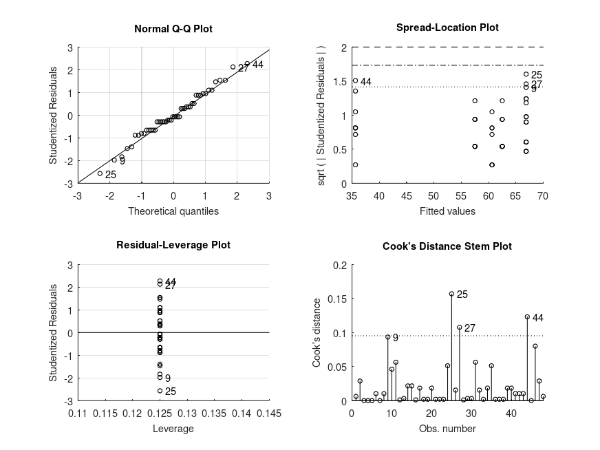
 % Unbalanced two-way design (2x2). The data is from a study on the effects
 % of gender and a college degree on starting salaries of a sample of company
 % employees, in Maxwell, Delaney and Kelly (2018): Chapter 7, Table 15. The
 % starting salaries are in units of 1000 dollars per annum.

 salary = [24 26 25 24 27 24 27 23 15 17 20 16, ...
           25 29 27 19 18 21 20 21 22 19]';
 gender = {'f' 'f' 'f' 'f' 'f' 'f' 'f' 'f' 'f' 'f' 'f' 'f'...
           'm' 'm' 'm' 'm' 'm' 'm' 'm' 'm' 'm' 'm'}';
 degree = [true true true true true true true true false false false false ...
           true true true false false false false false false false]';

 % ANOVA (including the main effect of gender averaged over all levels of
 % degree). In this order, the variability in salary only attributed to
 % having a degree is tested first. Then, having accounted for any effect of
 % degree, we test for whether variability in salary attributed to gender is
 % significant. Finally, the interaction term tests whether the effect of
 % gender differs depending on whether the subjects have a degree or not.
 [STATS, BOOTSTAT, AOVSTAT] = bootlm (salary, {degree, gender}, 'model', ...
                             'full', 'display', 'off', 'varnames', ...
                             {'degree', 'gender'}, 'seed', 1);

 fprintf ('ANOVA SUMMARY with gender averaged over levels of degree\n')
 for i = 1:numel(AOVSTAT.F)
   fprintf ('F = %.2f, p = %.3g for the model: %s\n', ...
            AOVSTAT.F(i), AOVSTAT.PVAL(i), AOVSTAT.MODEL{i});
 end

 % Since the interaction is not significant (F(1,18) = 0.42, p = 0.568), we
 % draw our attention to the main effects. We see that employees in this
 % have significantly different starting salaries depending or not on whether
 % they have a degree (F(1,18) = 87.20, p < 0.0001). We can also see that once
 % we factor in any differences in salary attributed to having a degree,
 % there is a significant difference in the salaries of men and women at
 % this company (F(1,18) = 10.97, p = 0.00893).

 % ANOVA (including the main effect of degree averaged over all levels of
 % gender). In this order, the variability in salary only attributed to being
 % male or female is tested first. Then, having accounted for any effect of
 % gender, we test for whether variability in salary attributed to having a
 % degree is significant. Finally, the interaction term tests whether the
 % effect of having a degree or not differs depending on whether the subjects
 % are male or female. (Note that the result for the interaction is not
 % affected by the order of the predictors).

 [STATS, BOOTSTAT, AOVSTAT] = bootlm (salary, {gender, degree}, 'model', ...
                             'full', 'display', 'off', 'varnames', ...
                             {'gender', 'degree'}, 'seed', 1);

 fprintf ('\nANOVA SUMMARY with degree averaged over levels of gender\n')
 for i = 1:numel(AOVSTAT.F)
   fprintf ('F = %.2f, p = %.3g for the model: %s\n', ...
            AOVSTAT.F(i), AOVSTAT.PVAL(i), AOVSTAT.MODEL{i});
 end

 % We can now see in the output that there is no significant difference in
 % salary between men and women in this company! (F(1,18) = 0.11, p = 0.755).
 % Why the discrepancy? There still seems to be a significant effect of
 % having a degree on the salary of people in this company (F(1,18) = 98.06,
 % p < 0.001). Lets look at the regression coefficients to see what this
 % effect of degree is.

 STATS = bootlm (salary, {gender, degree}, 'model', 'full', ...
                             'display', 'on', 'varnames', ...
                             {'gender', 'degree'}, 'method', 'bayesian', ...
                              'contrasts', 'treatment');
 STATS.levels

 % The order of the factor levels for degree indicates that having a degree
 % (i.e. a code of 1) is listed first and therefore is the reference level
 % for our treatment contrast coding. We see then from the second regression
 % coefficient that starting salaries in this company are $8K lower for
 % employees without a college degree. Let's now take a look at the estimated
 % marginal means.

 STATS = bootlm (salary, {gender, degree}, 'model', 'full', ...
                            'display', 'on', 'varnames', ...
                            {'gender', 'degree'}, 'dim', [1, 2], ...
                            'method', 'bayesian','prior', 'auto');

 % Ah ha! So it seems that sample sizes are very unbalanced here, with most
 % of the women in this sample having a degree, while most of the men not.
 % Since the regression coefficient indicated that a high starting salary is
 % an outcome of having a degree, this observation likely explains why
 % salaries where not significantly different between men and women when we
 % ran the ANOVA with gender listed first in the model (i.e. not accounting
 % for whether employees had a college degree). Note that our inferences here
 % assume that the unbalanced samples sizes are representative of similar
 % imbalance in the company as a whole (i.e. the population).

 % Since the interaction term (F(1,18) = 0.42) was not significant (p > 0.1),
 % we might rather consider the hypotheses tested using type II sums-of-
 % squares without the interaction, which do not depend on the order and have
 % more power respectively. This is easy to achieve with only 2 predictors,
 % by repeating the 'bootlm' commands with different predictors added last to
 % the model (as above) but without any interaction (i.e. setting 'model',
 % 'linear'). We then take the statistics for the last main effect listed
 % in each of the ANOVA tables - these then correspond to the ANOVA test for
 % the respective predictor with type II sums-of-squares. For example:

 [~, ~, AOVSTAT1] = bootlm (salary, {degree, gender}, 'model', ...
                             'linear', 'display', 'off', 'varnames', ...
                             {'degree', 'gender'}, 'seed', 1);

 fprintf ('\nANOVA SUMMARY (with type II sums-of-squares for main effects)\n')
 fprintf ('F = %.2f, p = %.3g for the model: %s (gender)\n', ...
          AOVSTAT1.F(2), AOVSTAT1.PVAL(2), AOVSTAT1.MODEL{2});

 [~, ~, AOVSTAT2] = bootlm (salary, {gender, degree}, 'model', ...
                             'linear', 'display', 'off', 'varnames', ...
                             {'gender', 'degree'}, 'seed', 1);

 fprintf ('F = %.2f, p = %.3g for the model: %s (degree)\n', ...
          AOVSTAT2.F(2), AOVSTAT2.PVAL(2), AOVSTAT2.MODEL{2});

 % Here is the output from 'anovan' for comparison:
 % ANOVA TABLE (Type II sums-of-squares):
 %
 % Source             Sum Sq.    d.f.    Mean Sq.  R Sq.            F  Prob>F
 % --------------------------------------------------------------------------
 % gender              30.462       1      30.462  0.373        11.31    .003
 % degree              272.39       1      272.39  0.842       101.13   <.001
 % Error               51.175      19      2.6934
 % Total               323.86      21
Produces the following output
ANOVA SUMMARY with gender averaged over levels of degree
F = 87.20, p = 0.0001 for the model: salary ~ 1 + degree
F = 10.97, p = 0.0089 for the model: salary ~ 1 + degree + gender
F = 0.42, p = 0.568 for the model: salary ~ 1 + degree + gender + degree:gender

ANOVA SUMMARY with degree averaged over levels of gender
F = 0.11, p = 0.755 for the model: salary ~ 1 + gender
F = 98.06, p = 0.0001 for the model: salary ~ 1 + gender + degree
F = 0.42, p = 0.568 for the model: salary ~ 1 + gender + degree + gender:degree

MODEL FORMULA (based on Wilkinson's notation):

salary ~ 1 + gender + degree + gender:degree

MODEL COEFFICIENTS

name                                   coeff       CI_lower    CI_upper
--------------------------------------------------------------------------------
(Intercept)                            +25.00      +24.04      +26.05
gender_1                               +2.000      +0.07344    +4.055
degree_1                               -8.000      -10.05      -5.931
gender:degree_1                        +1.000      -1.913      +3.842

ans =
{
  [1,1] =
  {
    [1,1] = f
    [2,1] = m
  }

  [2,1] =
  {
    [1,1] = 1
    [2,1] = 0
  }

}


MODEL FORMULA (based on Wilkinson's notation):

salary ~ 1 + gender + degree + gender:degree

MODEL ESTIMATED MARGINAL MEANS

name                                   mean        CI_lower    CI_upper        N
--------------------------------------------------------------------------------
f, 1                                   +25.00      +24.03      +26.07          8
m, 1                                   +27.00      +25.11      +29.00          3
f, 0                                   +17.00      +15.20      +19.22          4
m, 0                                   +20.00      +19.02      +21.03          7


ANOVA SUMMARY (with type II sums-of-squares for main effects)
F = 11.31, p = 0.0072 for the model: salary ~ 1 + degree + gender (gender)
F = 101.13, p = 0.0001 for the model: salary ~ 1 + gender + degree (degree)
and the following figure
| Figure 1 |
|---|
 |
Demonstration 8
The following code
% Simple linear regression. The data represents salaries of employees and
% their years of experience, modified from Allena Venkata. The salaries are
% in units of 1000 dollars per annum.
years = [1.20 1.40 1.60 2.10 2.30 3.00 3.10 3.30 3.30 3.80 4.00 4.10 ...
4.10 4.20 4.60 5.00 5.20 5.40 6.00 6.10 6.90 7.20 8.00 8.30 ...
8.80 9.10 9.60 9.70 10.40 10.60]';
salary = [39 46 38 44 40 57 60 54 64 57 63 56 57 57 61 68 66 83 81 94 92 ...
98 101 114 109 106 117 113 122 122]';
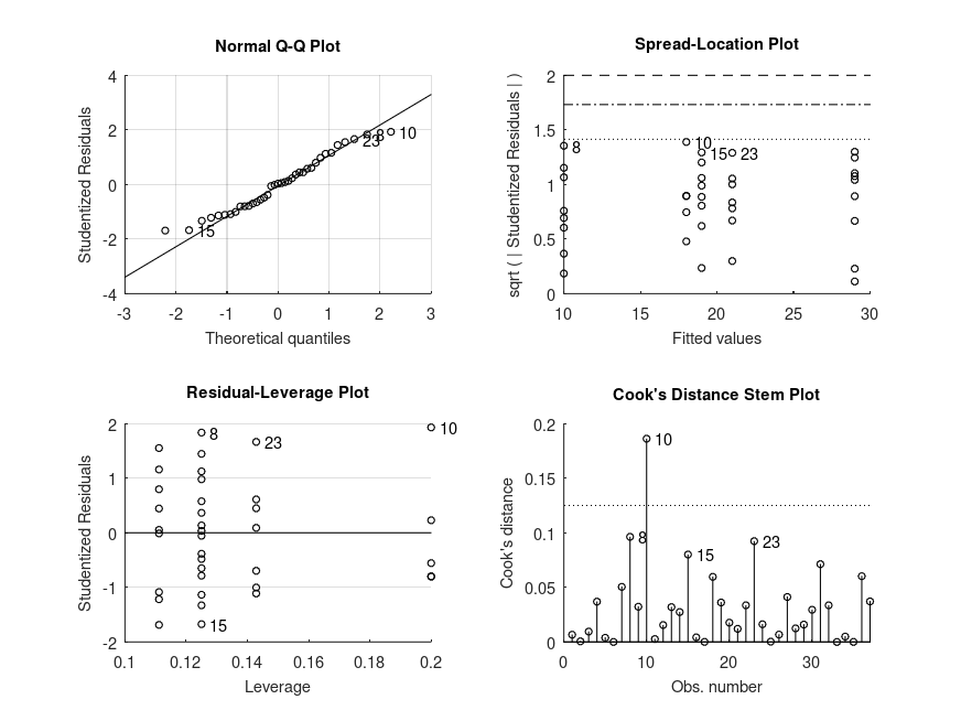
STATS = bootlm (salary, years, 'model', 'linear', 'continuous', 1, ...
'display', 'on', 'varnames', 'years');
% We can see from the intercept that the starting starting salary is $24.8 K
% and that salary increase per year of experience is $9.5 K.
Produces the following output
MODEL FORMULA (based on Wilkinson's notation):

salary ~ 1 + years

MODEL COEFFICIENTS

name                                   coeff       CI_lower    CI_upper    p-val
--------------------------------------------------------------------------------
(Intercept)                            +24.78      +20.44      +29.13      <.001
years                                  +9.455      +8.843      +10.07      <.001
and the following figure
| Figure 1 |
|---|
 |
Demonstration 9
The following code
 % One-way design with continuous covariate. The data is from a study of the
 % additive effects of species and temperature on chirpy pulses of crickets,
 % from Stitch, The Worst Stats Text eveR

 pulse = [67.9 65.1 77.3 78.7 79.4 80.4 85.8 86.6 87.5 89.1 ...
          98.6 100.8 99.3 101.7 44.3 47.2 47.6 49.6 50.3 51.8 ...
          60 58.5 58.9 60.7 69.8 70.9 76.2 76.1 77 77.7 84.7]';
 temp = [20.8 20.8 24 24 24 24 26.2 26.2 26.2 26.2 28.4 ...
         29 30.4 30.4 17.2 18.3 18.3 18.3 18.9 18.9 20.4 ...
         21 21 22.1 23.5 24.2 25.9 26.5 26.5 26.5 28.6]';
 species = {'ex' 'ex' 'ex' 'ex' 'ex' 'ex' 'ex' 'ex' 'ex' 'ex' 'ex' ...
            'ex' 'ex' 'ex' 'niv' 'niv' 'niv' 'niv' 'niv' 'niv' 'niv' ...
            'niv' 'niv' 'niv' 'niv' 'niv' 'niv' 'niv' 'niv' 'niv' 'niv'};

 % Perform ANCOVA (type I sums-of-squares)
 % Use 'anova' contrasts so that the continuous covariate is centered
 [STATS, BOOTSTAT, AOVSTAT] = bootlm (pulse, {temp, species}, 'model', ...
                           'linear', 'continuous', 1, 'display', 'off', ...
                           'varnames', {'temp', 'species'}, ...
                           'contrasts', 'anova', 'seed', 1);

 fprintf ('\nANCOVA SUMMARY (with type I sums-of-squares)\n')
 for i = 1:numel(AOVSTAT.F)
   fprintf ('F = %.2f, p = %.3g for the model: %s\n', ...
            AOVSTAT.F(i), AOVSTAT.PVAL(i), AOVSTAT.MODEL{i});
 end

 % Perform ANCOVA (type II sums-of-squares)
 % Use 'anova' contrasts so that the continuous covariate is centered
 [~, ~, AOVSTAT1] = bootlm (pulse, {temp, species}, 'model', ...
                           'linear', 'continuous', 1, 'display', 'off', ...
                           'varnames', {'temp', 'species'}, ...
                           'contrasts', 'anova', 'seed', 1);

 fprintf ('\nANOVA SUMMARY (with type II sums-of-squares)\n')
 fprintf ('F = %.2f, p = %.3g for the model: %s (species)\n', ...
          AOVSTAT1.F(2), AOVSTAT1.PVAL(2), AOVSTAT1.MODEL{2});

 [~, ~, AOVSTAT2] = bootlm (pulse, {species, temp}, 'model', ...
                           'linear', 'continuous', 2, 'display', 'off', ...
                           'varnames', {'species', 'temp'}, ...
                           'contrasts', 'anova', 'seed', 1);

 fprintf ('F = %.2f, p = %.3g for the model: %s (temp)\n', ...
          AOVSTAT2.F(2), AOVSTAT2.PVAL(2), AOVSTAT2.MODEL{2});

 % Estimate regression coefficients using 'anova' contrast coding
 STATS = bootlm (pulse, {temp, species}, 'model', 'linear', ...
                           'continuous', 1, 'display', 'on', ...
                           'varnames', {'temp', 'species'}, ...
                           'contrasts', 'anova');

 % 95% confidence intervals and p-values for the differences in the mean of
 % chirpy pulses of ex ad niv species (computed by wild bootstrap).
 STATS = bootlm (pulse, {temp, species}, 'model', 'linear', ...
                           'continuous', 1, 'display', 'on', ...
                           'varnames', {'temp', 'species'}, 'dim', 2, ...
                           'posthoc', 'trt_vs_ctrl', 'contrasts', 'anova');

 % 95% credible intervals for the estimated marginal means of chirpy pulses
 % of ex and niv species (computed by Bayesian bootstrap).
 STATS = bootlm (pulse, {temp, species}, 'model', 'linear', ...
                           'continuous', 1, 'display', 'on', ...
                           'varnames', {'temp', 'species'}, 'dim', 2, ...
                           'method', 'bayesian', 'prior', 'auto', ...
                           'contrasts', 'anova');
Produces the following output
ANCOVA SUMMARY (with type I sums-of-squares)
F = 2474.04, p = 0.0001 for the model: pulse ~ 1 + temp
F = 187.40, p = 0.0001 for the model: pulse ~ 1 + temp + species

ANOVA SUMMARY (with type II sums-of-squares)
F = 187.40, p = 0.0001 for the model: pulse ~ 1 + temp + species (species)
F = 1371.35, p = 0.0001 for the model: pulse ~ 1 + species + temp (temp)

MODEL FORMULA (based on Wilkinson's notation):

pulse ~ 1 + temp + species

MODEL COEFFICIENTS

name                                   coeff       CI_lower    CI_upper    p-val
--------------------------------------------------------------------------------
(Intercept)                            +73.37      +72.70      +74.05      <.001
temp                                   +3.603      +3.407      +3.799      <.001
species_1                              -10.07      -11.41      -8.725      <.001


MODEL FORMULA (based on Wilkinson's notation):

pulse ~ 1 + temp + species

MODEL POSTHOC COMPARISONS

name                                   mean        CI_lower    CI_upper    p-adj
--------------------------------------------------------------------------------
niv - ex                               -10.07      -11.41      -8.716      <.001


MODEL FORMULA (based on Wilkinson's notation):

pulse ~ 1 + temp + species

MODEL ESTIMATED MARGINAL MEANS

name                                   mean        CI_lower    CI_upper        N
--------------------------------------------------------------------------------
ex                                     +78.41      +77.43      +79.39         14
niv                                    +68.34      +67.61      +69.17         17
and the following figure
| Figure 1 |
|---|
 |
Demonstration 10
The following code
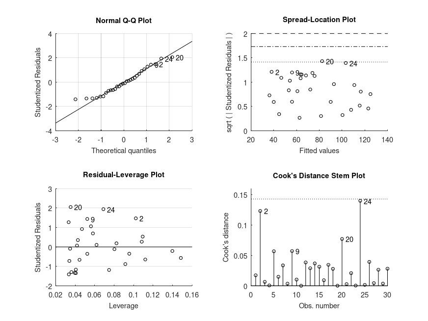
 % Unbalanced three-way design (3x2x2). The data is from a study of the
 % effects of three different drugs, biofeedback and diet on patient blood
 % pressure, adapted* from Maxwell, Delaney and Kelly (2018): Ch 8, Table 12

 drug = {'X' 'X' 'X' 'X' 'X' 'X' 'X' 'X' 'X' 'X' 'X' 'X' ...
         'X' 'X' 'X' 'X' 'X' 'X' 'X' 'X' 'X' 'X' 'X' 'X';
         'Y' 'Y' 'Y' 'Y' 'Y' 'Y' 'Y' 'Y' 'Y' 'Y' 'Y' 'Y' ...
         'Y' 'Y' 'Y' 'Y' 'Y' 'Y' 'Y' 'Y' 'Y' 'Y' 'Y' 'Y';
         'Z' 'Z' 'Z' 'Z' 'Z' 'Z' 'Z' 'Z' 'Z' 'Z' 'Z' 'Z' ...
         'Z' 'Z' 'Z' 'Z' 'Z' 'Z' 'Z' 'Z' 'Z' 'Z' 'Z' 'Z'};
 feedback = [1 1 1 1 1 1 1 1 1 1 1 1 0 0 0 0 0 0 0 0 0 0 0 0;
             1 1 1 1 1 1 1 1 1 1 1 1 0 0 0 0 0 0 0 0 0 0 0 0;
             1 1 1 1 1 1 1 1 1 1 1 1 0 0 0 0 0 0 0 0 0 0 0 0];
 diet = [0 0 0 0 0 0 1 1 1 1 1 1 0 0 0 0 0 0 1 1 1 1 1 1;
         0 0 0 0 0 0 1 1 1 1 1 1 0 0 0 0 0 0 1 1 1 1 1 1;
         0 0 0 0 0 0 1 1 1 1 1 1 0 0 0 0 0 0 1 1 1 1 1 1];
 BP = [170 175 165 180 160 158 161 173 157 152 181 190 ...
       173 194 197 190 176 198 164 190 169 164 176 175;
       186 194 201 215 219 209 164 166 159 182 187 174 ...
       189 194 217 206 199 195 171 173 196 199 180 203;
       180 187 199 170 204 194 162 184 183 156 180 173 ...
       202 228 190 206 224 204 205 199 170 160 179 179];

 % Perform 3-way ANOVA (this design is balanced, thus the order of predictors
 % does not make any difference)
 [STATS, BOOTSTAT, AOVSTAT] = bootlm (BP, {diet, drug, feedback}, 'seed', ...
                                    1, 'model', 'full', 'display', 'off', ...
                                    'varnames', {'diet', 'drug', 'feedback'});

 fprintf ('ANOVA SUMMARY\n')
 for i = 1:numel(AOVSTAT.F)
   fprintf ('F = %.2f, p = %.3g for the model: %s\n', ...
            AOVSTAT.F(i), AOVSTAT.PVAL(i), AOVSTAT.MODEL{i});
 end

 % Check regression coefficient corresponding to drug x feedback x diet
 STATS = bootlm (BP, {diet, drug, feedback}, 'model', 'full', ...
                                    'display', 'on', ...
                                    'varnames', {'diet', 'drug', 'feedback'});

 % 95% confidence intervals and p-values for the differences in mean salary
 % between males and females (computed by wild bootstrap).
 STATS = bootlm (BP, {diet, drug, feedback}, 'model', 'full', ...
                                    'display', 'on', 'dim', [1,2,3], ...
                                    'posthoc', 'trt_vs_ctrl', ...
                                    'varnames', {'diet', 'drug', 'feedback'});

 % 95% credible intervals for the estimated marginal means of salaries of
 % females and males (computed by Bayesian bootstrap).
 STATS = bootlm (BP, {diet, drug, feedback}, 'model', 'full', ...
                                    'display', 'on', 'dim', [1,2,3], ...
                                    'method', 'bayesian', 'prior', 'auto', ...
                                    'varnames', {'diet', 'drug', 'feedback'});
Produces the following output
ANOVA SUMMARY
F = 33.20, p = 0.0001 for the model: BP ~ 1 + diet
F = 11.73, p = 0.0002 for the model: BP ~ 1 + diet + drug
F = 13.07, p = 0.0009 for the model: BP ~ 1 + diet + drug + feedback
F = 2.88, p = 0.062 for the model: BP ~ 1 + diet + drug + feedback + diet:drug
F = 0.20, p = 0.64 for the model: BP ~ 1 + diet + drug + feedback + diet:drug + diet:feedback
F = 0.83, p = 0.436 for the model: BP ~ 1 + diet + drug + feedback + diet:drug + diet:feedback + drug:feedback
F = 3.43, p = 0.0398 for the model: BP ~ 1 + diet + drug + feedback + diet:drug + diet:feedback + drug:feedback + diet:drug:feedback

MODEL FORMULA (based on Wilkinson's notation):

BP ~ 1 + diet + drug + feedback + diet:drug + diet:feedback + drug:feedback + diet:drug:feedback

MODEL COEFFICIENTS

name                                   coeff       CI_lower    CI_upper    p-val
--------------------------------------------------------------------------------
(Intercept)                            +168.0      +157.9      +178.1      <.001
diet_1                                 +1.000      -15.70      +17.70       .883
drug_1                                 +36.00      +21.99      +50.01      <.001
drug_2                                 +21.00      +6.751      +35.25       .008
feedback_1                             +20.00      +7.057      +32.94       .006
diet:drug_1                            -33.00      -53.28      -12.72       .004
diet:drug_2                            -17.00      -37.94      +3.936       .104
diet:feedback_1                        -16.00      -35.17      +3.172       .095
drug:feedback_1                        -24.00      -42.08      -5.922       .011
drug:feedback_2                        -7.598e-16  -19.93      +19.93      1.000
diet:drug:feedback_1                   +35.00      +7.926      +62.07       .013
diet:drug:feedback_2                   +5.000      -24.39      +34.39       .737


MODEL FORMULA (based on Wilkinson's notation):

BP ~ 1 + diet + drug + feedback + diet:drug + diet:feedback + drug:feedback + diet:drug:feedback

MODEL POSTHOC COMPARISONS

name                                   mean        CI_lower    CI_upper    p-adj
--------------------------------------------------------------------------------
1, X, 1 - 0, X, 1                      +1.000      -15.45      +17.45       .887
0, Y, 1 - 0, X, 1                      +36.00      +21.52      +50.48       .003
1, Y, 1 - 0, X, 1                      +4.000      -8.896      +16.90       .779
0, Z, 1 - 0, X, 1                      +21.00      +6.775      +35.22       .062
1, Z, 1 - 0, X, 1                      +5.000      -8.547      +18.55       .813
0, X, 0 - 0, X, 1                      +20.00      +7.164      +32.84       .054
1, X, 0 - 0, X, 1                      +5.000      -6.615      +16.62       .813
0, Y, 0 - 0, X, 1                      +32.00      +20.00      +44.00       .003
1, Y, 0 - 0, X, 1                      +19.00      +2.687      +35.31       .124
0, Z, 0 - 0, X, 1                      +41.00      +25.53      +56.47       .003
1, Z, 0 - 0, X, 1                      +14.00      -4.969      +32.97       .411


MODEL FORMULA (based on Wilkinson's notation):

BP ~ 1 + diet + drug + feedback + diet:drug + diet:feedback + drug:feedback + diet:drug:feedback

MODEL ESTIMATED MARGINAL MEANS

name                                   mean        CI_lower    CI_upper        N
--------------------------------------------------------------------------------
0, X, 1                                +168.0      +161.3      +174.6          6
1, X, 1                                +169.0      +158.0      +181.0          6
0, Y, 1                                +204.0      +193.6      +213.5          6
1, Y, 1                                +172.0      +163.9      +180.9          6
0, Z, 1                                +189.0      +178.8      +198.8          6
1, Z, 1                                +173.0      +163.5      +181.1          6
0, X, 0                                +188.0      +179.6      +196.0          6
1, X, 0                                +173.0      +165.7      +181.0          6
0, Y, 0                                +200.0      +192.6      +208.4          6
1, Y, 0                                +187.0      +176.1      +197.4          6
0, Z, 0                                +209.0      +198.1      +220.9          6
1, Z, 0                                +182.0      +169.3      +196.4          6
and the following figure
| Figure 1 |
|---|
 |
Demonstration 11
The following code
% Factorial design with continuous covariate. The data is from a study of
% the effects of treatment and exercise on stress reduction score after
% adjusting for age. Data from R datarium package).
score = [95.6 82.2 97.2 96.4 81.4 83.6 89.4 83.8 83.3 85.7 ...
97.2 78.2 78.9 91.8 86.9 84.1 88.6 89.8 87.3 85.4 ...
81.8 65.8 68.1 70.0 69.9 75.1 72.3 70.9 71.5 72.5 ...
84.9 96.1 94.6 82.5 90.7 87.0 86.8 93.3 87.6 92.4 ...
100. 80.5 92.9 84.0 88.4 91.1 85.7 91.3 92.3 87.9 ...
91.7 88.6 75.8 75.7 75.3 82.4 80.1 86.0 81.8 82.5]';
treatment = {'yes' 'yes' 'yes' 'yes' 'yes' 'yes' 'yes' 'yes' 'yes' 'yes' ...
'yes' 'yes' 'yes' 'yes' 'yes' 'yes' 'yes' 'yes' 'yes' 'yes' ...
'yes' 'yes' 'yes' 'yes' 'yes' 'yes' 'yes' 'yes' 'yes' 'yes' ...
'no' 'no' 'no' 'no' 'no' 'no' 'no' 'no' 'no' 'no' ...
'no' 'no' 'no' 'no' 'no' 'no' 'no' 'no' 'no' 'no' ...
'no' 'no' 'no' 'no' 'no' 'no' 'no' 'no' 'no' 'no'}';
exercise = {'lo' 'lo' 'lo' 'lo' 'lo' 'lo' 'lo' 'lo' 'lo' 'lo' ...
'mid' 'mid' 'mid' 'mid' 'mid' 'mid' 'mid' 'mid' 'mid' 'mid' ...
'hi' 'hi' 'hi' 'hi' 'hi' 'hi' 'hi' 'hi' 'hi' 'hi' ...
'lo' 'lo' 'lo' 'lo' 'lo' 'lo' 'lo' 'lo' 'lo' 'lo' ...
'mid' 'mid' 'mid' 'mid' 'mid' 'mid' 'mid' 'mid' 'mid' 'mid' ...
'hi' 'hi' 'hi' 'hi' 'hi' 'hi' 'hi' 'hi' 'hi' 'hi'}';
age = [59 65 70 66 61 65 57 61 58 55 62 61 60 59 55 57 60 63 62 57 ...
58 56 57 59 59 60 55 53 55 58 68 62 61 54 59 63 60 67 60 67 ...
75 54 57 62 65 60 58 61 65 57 56 58 58 58 52 53 60 62 61 61]';
% ANOVA/ANCOVA statistics
% Use 'anova' contrasts so that the continuous covariate is centered
[STATS, BOOTSTAT, AOVSTAT] = bootlm (score, {age, exercise, treatment}, ...
'model', [1 0 0; 0 1 0; 0 0 1; 0 1 1], ...
'continuous', 1, 'display', 'off', ...
'varnames', {'age', 'exercise', 'treatment'},...
'contrasts', 'anova');
fprintf ('ANOVA / ANCOVA SUMMARY\n')
for i = 1:numel(AOVSTAT.F)
fprintf ('F = %.2f, p = %.3g for the model: %s\n', ...
AOVSTAT.F(i), AOVSTAT.PVAL(i), AOVSTAT.MODEL{i});
end
% Estimate regression coefficients
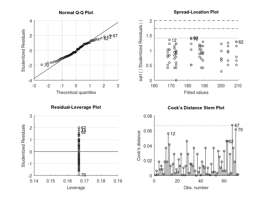
STATS = bootlm (score, {age, exercise, treatment}, ...
'model', [1 0 0; 0 1 0; 0 0 1; 0 1 1], ...
'continuous', 1, 'display', 'on', ...
'varnames', {'age', 'exercise', 'treatment'}, ...
'contrasts', 'anova');
% 95% confidence intervals and p-values for the differences in mean score
% across different treatments and amounts of exercise after adjusting for
STATS = bootlm (score, {age, exercise, treatment}, ...
'model', [1 0 0; 0 1 0; 0 0 1; 0 1 1], ...
'continuous', 1, 'display', 'on', ...
'varnames', {'age', 'exercise', 'treatment'}, ...
'dim', [2, 3], 'posthoc', 'trt_vs_ctrl', ...
'contrasts', 'anova');
% 95% credible intervals for the estimated marginal means of scores across
% different treatments and amounts of exercise after adjusting for age
% (computed by Bayesian bootstrap).
STATS = bootlm (score, {age, exercise, treatment}, 'dim', [2, 3], ...
'model', [1 0 0; 0 1 0; 0 0 1; 0 1 1], ...
'continuous', 1, 'display', 'on', ...
'varnames', {'age', 'exercise', 'treatment'}, ...
'method', 'bayesian', 'prior', 'auto', ...
'contrasts', 'anova');
Produces the following output
ANOVA / ANCOVA SUMMARY
F = 44.02, p = 0.0001 for the model: score ~ 1 + age
F = 19.74, p = 0.0001 for the model: score ~ 1 + age + exercise
F = 11.10, p = 0.0022 for the model: score ~ 1 + age + exercise + treatment
F = 4.45, p = 0.0154 for the model: score ~ 1 + age + exercise + treatment + exercise:treatment

MODEL FORMULA (based on Wilkinson's notation):

score ~ 1 + age + exercise + treatment + exercise:treatment

MODEL COEFFICIENTS

name                                   coeff       CI_lower    CI_upper    p-val
--------------------------------------------------------------------------------
(Intercept)                            +84.58      +83.29      +85.86      <.001
age                                    +0.5036     +0.1874     +0.8197      .003
exercise_1                             +0.09497    -3.118      +3.308       .955
exercise_2                             -9.594      -12.82      -6.364      <.001
treatment_1                            +4.320      +1.715      +6.924       .002
exercise:treatment_1                   +0.1550     -6.387      +6.697       .961
exercise:treatment_2                   +8.218      +1.728      +14.71       .014


MODEL FORMULA (based on Wilkinson's notation):

score ~ 1 + age + exercise + treatment + exercise:treatment

MODEL POSTHOC COMPARISONS

name                                   mean        CI_lower    CI_upper    p-adj
--------------------------------------------------------------------------------
mid, yes - lo, yes                     +0.01746    -5.617      +5.652       .995
hi, yes - lo, yes                      -13.70      -18.46      -8.949      <.001
lo, no - lo, yes                       +1.529      -3.395      +6.452       .763
mid, no - lo, yes                      +1.701      -3.195      +6.597       .763
hi, no - lo, yes                       -3.957      -9.130      +1.217       .332


MODEL FORMULA (based on Wilkinson's notation):

score ~ 1 + age + exercise + treatment + exercise:treatment

MODEL ESTIMATED MARGINAL MEANS

name                                   mean        CI_lower    CI_upper        N
--------------------------------------------------------------------------------
lo, yes                                +86.98      +83.41      +90.50         10
mid, yes                               +87.00      +83.28      +90.37         10
hi, yes                                +73.28      +70.48      +76.11         10
lo, no                                 +88.51      +86.06      +91.44         10
mid, no                                +88.68      +86.27      +91.09         10
hi, no                                 +83.02      +79.72      +86.48         10
and the following figure
| Figure 1 |
|---|
 |
Demonstration 12
The following code
% Unbalanced one-way design with custom, orthogonal contrasts. Data from
% www.uvm.edu/~statdhtx/StatPages/Unequal-ns/Unequal_n%27s_contrasts.html
dv = [ 8.706 10.362 11.552 6.941 10.983 10.092 6.421 14.943 15.931 ...
22.968 18.590 16.567 15.944 21.637 14.492 17.965 18.851 22.891 ...
22.028 16.884 17.252 18.325 25.435 19.141 21.238 22.196 18.038 ...
22.628 31.163 26.053 24.419 32.145 28.966 30.207 29.142 33.212 ...
25.694 ]';
g = [1 1 1 1 1 1 1 1 2 2 2 2 2 3 3 3 3 3 3 3 3 ...
4 4 4 4 4 4 4 5 5 5 5 5 5 5 5 5]';
C = [ 0.4001601 0.3333333 0.5 0.0
0.4001601 0.3333333 -0.5 0.0
0.4001601 -0.6666667 0.0 0.0
-0.6002401 0.0000000 0.0 0.5
-0.6002401 0.0000000 0.0 -0.5];
% 95% confidence intervals and p-values for linear contrasts
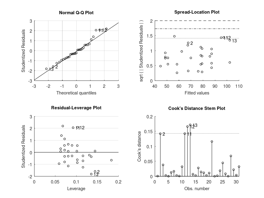
STATS = bootlm (dv, g, 'contrasts', C, 'varnames', 'score', ...
'alpha', 0.05, 'display', true);
% 95% credible intervals for estimated marginal means
STATS = bootlm (dv, g, 'contrasts', C, 'varnames', 'score', ...
'alpha', 0.05, 'display', true, 'dim', 1, ...
'method', 'Bayesian', 'prior', 'auto');
Produces the following output
MODEL FORMULA (based on Wilkinson's notation):

dv ~ 1 + score

MODEL COEFFICIENTS

name                                   coeff       CI_lower    CI_upper    p-val
--------------------------------------------------------------------------------
(Intercept)                            +19.40      +18.42      +20.38      <.001
score_1                                -9.330      -11.30      -7.359      <.001
score_2                                -5.000      -7.877      -2.123       .002
score_3                                -8.000      -11.50      -4.500      <.001
score_4                                -8.000      -11.04      -4.958      <.001


MODEL FORMULA (based on Wilkinson's notation):

dv ~ 1 + score

MODEL ESTIMATED MARGINAL MEANS

name                                   mean        CI_lower    CI_upper        N
--------------------------------------------------------------------------------
1                                      +10.00      +8.169      +11.90          8
2                                      +18.00      +16.01      +20.71          5
3                                      +19.00      +17.02      +21.06          8
4                                      +21.00      +19.01      +22.93          7
5                                      +29.00      +26.94      +30.90          9
and the following figure
| Figure 1 |
|---|
 |
Demonstration 13
The following code
 % Analysis of nested one-way ANOVA design using clustered resampling.
 %
 % While the effect of nesting is minimal on parameter estimates, it can have
 % a big effect on standard errors, confidence intervals and p-values for the
 % parameters. One way to estimate p-values and the precision of parameter
 % estimates for fixed effects in nested designs is to fit a mixed linear
 % model. Another way, as we do so here, is to fit a linear model using
 % bootstrap with clustered resampling.

 % Nested model example from:
 % https://www.southampton.ac.uk/~cpd/anovas/datasets/#Chapter2

 data = [4.5924 7.3809 21.322; -0.5488 9.2085 25.0426; ...
         6.1605 13.1147 22.66; 2.3374 15.2654 24.1283; ...
         5.1873 12.4188 16.5927; 3.3579 14.3951 10.2129; ...
         6.3092 8.5986 9.8934; 3.2831 3.4945 10.0203];

 clustid = [1 3 5; 1 3 5; 1 3 5; 1 3 5; ...
            2 4 6; 2 4 6; 2 4 6; 2 4 6];

 group = {'A' 'B' 'C'; 'A' 'B' 'C'; 'A' 'B' 'C'; 'A' 'B' 'C'; ...
          'A' 'B' 'C'; 'A' 'B' 'C'; 'A' 'B' 'C'; 'A' 'B' 'C'};

 [STATS, BOOTSTAT, AOVSTAT] = bootlm (data, {group}, 'clustid', clustid, ...
                                      'seed', 1, 'display', 'off');

 fprintf ('ANOVA SUMMARY\n')
 fprintf ('F = %.2f, p = %.3g for the model: %s\n', ...
          AOVSTAT.F(1), AOVSTAT.PVAL(1), AOVSTAT.MODEL{1});
Produces the following output
ANOVA SUMMARY
F = 17.08, p = 0.0525 for the model: data ~ 1 + X1
Demonstration 14
The following code
 % Variations in design for two-way ANOVA (2x2) with interaction.

 % Arousal was measured in rodents assigned to four experimental groups in a
 % between-subjects design with two factors: group (lesion/control) and
 % stimulus (fearful/neutral). In this design, each rodent is allocated to one
 % combination of levels in group and stimulus, and a single measurment of
 % arousal is made. The question we are asking here is, does the effect of a
 % fear-inducing stimulus on arousal depend on whether or not rodents had a
 % lesion?

 group = {'control' 'control' 'control' 'control' 'control' 'control' ...
          'lesion'  'lesion'  'lesion'  'lesion'  'lesion'  'lesion'  ...
          'control' 'control' 'control' 'control' 'control' 'control' ...
          'lesion'  'lesion'  'lesion'  'lesion'  'lesion'  'lesion'};

 stimulus = {'fearful' 'fearful' 'fearful' 'fearful' 'fearful' 'fearful' ...
             'fearful' 'fearful' 'fearful' 'fearful' 'fearful' 'fearful' ...
             'neutral' 'neutral' 'neutral' 'neutral' 'neutral' 'neutral' ...
             'neutral' 'neutral' 'neutral' 'neutral' 'neutral' 'neutral'};

 arousal = [0.78 0.86 0.65 0.83 0.78 0.81 0.65 0.69 0.61 0.65 0.59 0.64 ...
            0.54 0.6 0.67 0.63 0.56 0.55 0.645 0.565 0.625 0.485 0.655 0.515];

 [stats, bootstat, aovstat] = bootlm (arousal, {group, stimulus}, ...
                                      'seed', 1, 'display', 'off', ...
                                      'model', 'full', ...
                                      'varnames', {'group', 'stimulus'});

 fprintf ('ANOVA SUMMARY for the between-subjects design.\n')
 for i = 1:numel(aovstat.F)
   fprintf ('F = %.2f, p = %.3g for the model: %s\n', ...
            aovstat.F(i), aovstat.PVAL(i), aovstat.MODEL{i});
 end

 % Lets consider having a mixed design with rodents allocated into control and
 % lesion groups but with two arousal measurements made for each rodent, the
 % first to a neutral stimulus and the second to a fearful stimulus. Thus, we
 % now need to introduce another variable, a random effect, which defines the
 % identity of the rodent of each measurement:

 id = [1 2 3 4 5 6 7 8 9 10 11 12 1 2 3 4 5 6 7 8 9 10 11 12];

 % Instead of fitting a non-linear mixed model, we will fit the same linear
 % model but use wild cluster bootstrap resambling to capture the dependence
 % structure in the data by providing the id variable to the 'clustid' input
 % argument.

 [stats, bootstat, aovstat] = bootlm (arousal, {group, stimulus}, ...
                                      'seed', 1, 'display', 'off', ...
                                      'model', 'full', ...
                                      'clustid', id, ...
                                      'varnames', {'group', 'stimulus'});

 fprintf ('\nANOVA SUMMARY for the mixed between/within subjects design.\n')
 for i = 1:numel(aovstat.F)
   fprintf ('F = %.2f, p = %.3g for the model: %s\n', ...
            aovstat.F(i), aovstat.PVAL(i), aovstat.MODEL{i});
 end
Produces the following output
ANOVA SUMMARY for the between-subjects design.
F = 10.36, p = 0.0093 for the model: arousal ~ 1 + group
F = 26.39, p = 0.0003 for the model: arousal ~ 1 + group + stimulus
F = 7.89, p = 0.0117 for the model: arousal ~ 1 + group + stimulus + group:stimulus

ANOVA SUMMARY for the mixed between/within subjects design.
F = 10.36, p = 0.0001 for the model: arousal ~ 1 + group
F = 26.39, p = 0.0071 for the model: arousal ~ 1 + group + stimulus
F = 7.89, p = 0.046 for the model: arousal ~ 1 + group + stimulus + group:stimulus
Demonstration 15
The following code
% Prediction errors and information criteria of linear models.
% Data from Table 9.1, on page 107 of Efron and Tibshirani (1993)
% An Introduction to the Bootstrap.
amount = [25.8; 20.5; 14.3; 23.2; 20.6; 31.1; 20.9; 20.9; 30.4; ...
16.3; 11.6; 11.8; 32.5; 32.0; 18.0; 24.1; 26.5; 25.8; ...
28.8; 22.0; 29.7; 28.9; 32.8; 32.5; 25.4; 31.7; 28.5];
hrs = [99; 152; 293; 155; 196; 53; 184; 171; 52; ...
376; 385; 402; 29; 76; 296; 151; 177; 209; ...
119; 188; 115; 88; 58; 49; 150; 107; 125];
lot = {'A'; 'A'; 'A'; 'A'; 'A'; 'A'; 'A'; 'A'; 'A'; ...
'B'; 'B'; 'B'; 'B'; 'B'; 'B'; 'B'; 'B'; 'B'; ...
'C'; 'C'; 'C'; 'C'; 'C'; 'C'; 'C'; 'C'; 'C'};
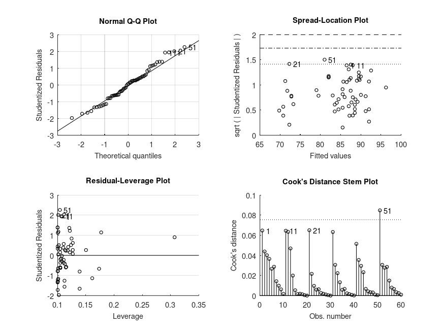
[STATS, BOOTSTAT, AOVSTAT, PRED_ERR] = bootlm (amount, {hrs, lot}, ...
'continuous', 1, 'seed', 1, ...
'model', 'linear', 'display', 'on', ...
'varnames', {'hrs', 'lot'}, ...
'contrasts', 'treatment');
fprintf ('PREDICTION ERROR of the FULL MODEL = %.2f\n', PRED_ERR.PE(3))
% Note: The value of prediction error is lower than the 3.00 calculated by
% Efron and Tibshirani (1993) using the same refined bootstrap procedure,
% because they have used case resampling whereas we have used wild bootstrap
% resampling. The equivalent value of Cp (eq. to AIC) statistic is 2.96.
PRED_ERR
% The results from the bootstrap are broadly consistent to the results
% obtained for Akaike's Information Criterion (AIC, computed in R with the
% AIC function from the 'stats' package):
%
% MODEL AIC EIC
% amount ~ 1 180.17 178.41
% amount ~ 1 + hrs 127.33 125.00
% amount ~ 1 + hrs + lot 107.85 106.36
Produces the following output
MODEL FORMULA (based on Wilkinson's notation):

amount ~ 1 + hrs + lot

MODEL COEFFICIENTS

name                                   coeff       CI_lower    CI_upper    p-val
--------------------------------------------------------------------------------
(Intercept)                            +32.13      +30.27      +34.00      <.001
hrs                                    -0.06014    -0.06841    -0.05186    <.001
lot_1                                  +3.973      +2.172      +5.775      <.001
lot_2                                  +3.466      +1.962      +4.970      <.001

PREDICTION ERROR of the FULL MODEL = 2.86
PRED_ERR =

  scalar structure containing the fields:

    MODEL =
    {
      [1,1] = amount ~ 1
      [2,1] = amount ~ 1 + hrs
      [3,1] = amount ~ 1 + hrs + lot
    }

    PE =

           42.937
           5.9086
           2.8582

    PRESS =

           1159.3
           159.53
           77.171

    RSQ_pred =

        -0.075489
            0.852
          0.92841

    EIC =

           178.41
              125
           106.36

    RL =

                1
        3.968e+11
       4.4286e+15

    Wt =

       2.2578e-16
       8.9592e-05
          0.99991
and the following figure
| Figure 1 |
|---|
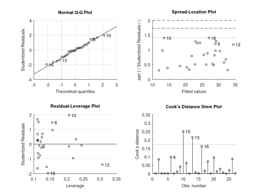 |
Demonstration 16
The following code
 % Step-wise regression

 sr = [11.43;12.07;13.17;05.75;12.88;08.79;00.60;11.90; ...
       04.98;10.78;16.85;03.59;11.24;12.64;12.55;10.67; ...
       03.01;07.70;01.27;09.00;11.34;14.28;21.10;03.98; ...
       10.35;15.48;10.25;14.65;10.67;07.30;04.44;02.02; ...
       12.70;12.78;12.49;11.14;13.30;11.77;06.86;14.13; ...
       05.13;02.81;07.81;07.56;09.22;18.56;07.72;09.24; ...
       08.89;4.71];

 pop15 = [29.35;23.32;23.80;41.89;42.19;31.72;39.74;44.75;
          46.64;47.64;24.42;46.31;27.84;25.06;23.31;25.62;
          46.05;47.32;34.03;41.31;31.16;24.52;27.01;41.74;
          21.80;32.54;25.95;24.71;32.61;45.04;43.56;41.18;
          44.19;46.26;28.96;31.94;31.92;27.74;21.44;23.49;
          43.42;46.12;23.27;29.81;46.40;45.25;41.12;28.13;
         43.69;47.20];

 pop75 = [2.87;4.41;4.43;1.67;0.83;2.85;1.34;0.67; ...
          1.06;1.14;3.93;1.19;2.37;4.70;3.35;3.10; ...
          0.87;0.58;3.08;0.96;4.19;3.48;1.91;0.91; ...
          3.73;2.47;3.67;3.25;3.17;1.21;1.20;1.05; ...
          1.28;1.12;2.85;2.28;1.52;2.87;4.54;3.73; ...
          1.08;1.21;4.46;3.43;0.90;0.56;1.73;2.72; ...
          2.07;0.66];

 dpi = [2329.68;1507.99;2108.47;0189.13;0728.47;2982.88;0662.86;0289.52; ...
        0276.65;0471.24;2496.53;0287.77;1681.25;2213.82;2457.12;0870.85; ...
        0289.71;0232.44;1900.10;0088.94;1139.95;1390.00;1257.28;0207.68; ...
        2449.39;0601.05;2231.03;1740.70;1487.52;0325.54;0568.56;0220.56; ...
        0400.06;0152.01;0579.51;0651.11;0250.96;0768.79;3299.49;2630.96; ...
        0389.66;0249.87;1813.93;4001.89;0813.39;0138.33;0380.47;0766.54; ...
        0123.58;0242.69];

 ddpi = [02.87;03.93;03.82;00.22;04.56;02.43;02.67;06.51;
         03.08;02.80;03.99;02.19;04.32;04.52;03.44;06.28;
         01.48;03.19;01.12;01.54;02.99;03.54;08.21;05.81;
         01.57;08.12;03.62;07.66;01.76;02.48;03.61;01.03;
         00.67;02.00;07.48;02.19;02.00;04.35;03.01;02.70;
         02.96;01.13;02.01;02.45;00.53;05.14;10.23;01.88;
         16.71;05.08];

  [STATS, BOOTSTAT, AOVSTAT, PRED_ERR] = bootlm (sr, {pop15, pop75, ...
                               dpi, ddpi}, 'seed', 1, 'continuous', [1:4], ...
                               'model', 'linear', 'display', 'off', ...
                               'varnames', {'pop15','pop75','dpi','ddpi'},
                               'contrasts', 'treatment');

 PRED_ERR

 % The results from the bootstrap are broadly consistent to the results
 % obtained for PE, PRESS and RSQ_pred using cross-validation:
 %
 %     MODEL                                   PE-CV    PRESS-CV  RSQ_pred-CV
 %     sr ~ 1                                  20.48    1024.186       -0.041
 %     sr ~ 1 + pop15                          16.88     843.910       +0.142
 %     sr ~ 1 + pop15 + pop75                  16.62     830.879       +0.155
 %     sr ~ 1 + pop15 + pop75 + dpi            16.54     827.168       +0.159
 %     sr ~ 1 + pop15 + pop75 + dpi + ddpi     15.98     798.939       +0.188


 % ANOVA p-values of the nested models
 AOVSTAT.PVAL

 % Relative likelihood of the nested models
 PRED_ERR.RL(2:end) ./ PRED_ERR.RL(1:end-1)
Produces the following output
PRED_ERR =

  scalar structure containing the fields:

    MODEL =
    {
      [1,1] = sr ~ 1
      [2,1] = sr ~ 1 + pop15
      [3,1] = sr ~ 1 + pop15 + pop75
      [4,1] = sr ~ 1 + pop15 + pop75 + dpi
      [5,1] = sr ~ 1 + pop15 + pop75 + dpi + ddpi
    }

    PE =

           20.477
             16.8
            16.34
            16.22
           15.191

    PRESS =

           1023.8
              840
           817.01
           811.02
           759.53

    RSQ_pred =

        -0.040869
          0.14602
          0.16939
          0.17548
          0.22783

    EIC =

           293.13
           283.41
           282.22
           281.92
           278.87

    RL =

                1
           129.42
           234.65
           271.81
           1254.4

    Wt =

       0.00052875
         0.068431
          0.12407
          0.14372
          0.66325


ans =

   0.00020002
      0.10891
      0.17192
     0.017102

ans =

       129.42
       1.8131
       1.1583
       4.6149
Package: statistics-resampling