bootridge
 Empirical Bayes penalized regression for univariate or multivariate outcomes,
 with shrinkage tuned to minimize prediction error computed by .632 bootstrap.

 -- Function File: bootridge (Y, X)
 -- Function File: bootridge (Y, X, CATEGOR)
 -- Function File: bootridge (Y, X, CATEGOR, NBOOT)
 -- Function File: bootridge (Y, X, CATEGOR, NBOOT, ALPHA)
 -- Function File: bootridge (Y, X, CATEGOR, NBOOT, ALPHA, L)
 -- Function File: bootridge (Y, X, CATEGOR, NBOOT, ALPHA, L, DEFF)
 -- Function File: bootridge (Y, X, CATEGOR, NBOOT, ALPHA, L, DEFF, SEED)
 -- Function File: bootridge (Y, X, CATEGOR, NBOOT, ALPHA, L, DEFF, SEED, TOL)
 -- Function File: S = bootridge (Y, X, ...)
 -- Function File: [S, YHAT] = bootridge (Y, X, ...)

      'bootridge (Y, X)' fits an empirical Bayes ridge regression model using
      a linear Normal (Gaussian) likelihood with an empirical Bayes normal
      ridge prior on the regression coefficients. The ridge tuning constant
      (lambda) is optimized via .632 bootstrap-based machine learning (ML) to
      minimize out-of-bag prediction error [1, 2]. Y is an m-by-q matrix of
      outcomes and X is an m-by-n design matrix whose first column must
      correspond to an intercept term. If an intercept term (a column of ones)
      is not found in the first column of X, one is added automatically. If any
      rows of X or Y contain missing values (NaN) or infinite values (+/- Inf),
      the corresponding observations are omitted before fitting.

      For each outcome, the function prints posterior summaries for regression
      coefficients or linear estimates, including posterior means, equal-tailed
      credible intervals, Bayes factors (lnBF10), and the marginal prior used
      for inference. When multiple outcomes are fitted (q > 1), the function
      additionally prints posterior summaries for the residual correlations
      between outcomes, reported as unique (lower-triangular) outcome pairs.
      For each correlation, the printed output includes the estimated
      correlation and its credible interval.

      Interpretation note (empirical Bayes):
        Bayes factors reported by 'bootridge' are empirical‑Bayes approximations
        based on a data‑tuned ridge prior. They are best viewed as model‑
        comparison diagnostics (evidence on a predictive, information‑theoretic
        scale) rather than literal posterior odds under a fully specified prior
        [3–5]. The log scale (lnBF10) is numerically stable and recommended
        for interpretation; BF10 may be shown as 0 or Inf when beyond machine
        range, while lnBF10 remains finite. These Bayesian statistics converge
        to standard conjugate Bayesian evidence as the effective residual
        degrees of freedom (df_t) increase.

      For convenience, the statistics-resampling package also provides the
      function `bootlm`, which offers a user-friendly but feature-rich interface
      for fitting univariate linear models with continuous and categorical
      predictors. The design matrix X and hypothesis matrix L returned in the
      MAT-file produced by `bootlm` can be supplied directly to `bootridge`.
      The outputs of `bootlm` also provide a consistent definition of the model
      coefficients, thereby facilitating interpretation of parameter estimates,
      contrasts, and posterior summaries. The design matrix X and hypothesis
      matrix L can also be obtained the same way with one of the outcomes of a
      multivariate data set, then fit to all the outcomes using bootridge.

      'bootridge (Y, X, CATEGOR)' specifies the predictor columns that
      correspond to categorical variables. CATEGOR must be a scalar or vector
      of integer column indices referring to columns of X (excluding the
      intercept). Alternatively, if all predictor terms are categorical, set
      CATEGOR to 'all' or '*'. CATEGOR does NOT create or modify dummy or
      contrast coding; users are responsible for supplying an appropriately
      coded design matrix X. The indices in CATEGOR are used to identify
      predictors that represent categorical variables, even when X is already
      coded, so that variance-based penalty scaling is not applied to these
      terms.

      For categorical predictors in ridge regression, use meaningful centered
      and preferably orthogonal (e.g. Helmert or polynomial) contrasts whenever
      possible, since shrinkage occurs column-wise in the coefficient basis.
      Orthogonality leads to more stable shrinkage and tuning of the ridge
      parameter. Although the prior is not rotationally invariant, Bayes
      factors for linear contrasts defined via a hypothesis matrix (L) are
      typically more stable when the contrasts defining the coefficients are
      orthogonal.

      'bootridge (Y, X, CATEGOR, NBOOT)' sets the number of bootstrap samples
      used to estimate the .632 bootstrap prediction error. The bootstrap* has
      first order balance to improve the efficiency for variance estimation,
      and utilizes bootknife (leave-one-out) resampling to guarantee
      observations in the out-of-bag samples. The default value of NBOOT is
      100, but more resamples are recommended to reduce monte carlo error.

      The bootstrap tuning of the ridge parameter relies on resampling
      functionality provided by the statistics-resampling package. In
      particular, `bootridge` depends on the functions `bootstrp` and `boot` to
      perform balanced bootstrap and bootknife (leave-one-out) resampling and
      generate out-of-bag samples. These functions are required for estimation
      of the .632 bootstrap prediction error used to select the ridge tuning
      constant.

      'bootridge (Y, X, CATEGOR, NBOOT, ALPHA)' sets the central mass of equal-
      tailed credibility intervals (CI) to (1 - ALPHA) with probability mass
      ALPHA/2 in each tail, and sets the threshold for the adjusted stability
      selection (SS) probabilities of the regression coefficients to (1 - ALPHA).
      ALPHA must be a scalar value between 0 and 1. The default value of ALPHA
      is 0.05 for 95% intervals.

      'bootridge (Y, X, CATEGOR, NBOOT, ALPHA, L)' specifies a hypothesis
      matrix L of size n-by-c defining c linear contrasts or model-based
      estimates of the regression coefficients. In this case, posterior
      summaries and credible intervals are reported for the linear estimates
      rather than the model coefficients.

      'bootridge (Y, X, CATEGOR, NBOOT, ALPHA, L, DEFF)' specifies a design
      effect used to account for clustering or dependence. DEFF inflates the
      posterior covariance and reduces the effective degrees of freedom (df_t)
      to ensure Bayes factors and intervals are calibrated for the effective
      sample size. For a mean, Kish's formula DEFF = 1+(g-1)*r (where g is
      cluster size) suggests an upper bound of g. However, for regression
      slopes, the realized DEFF depends on the predictor type: it can exceed
      g for between-cluster predictors or be less than 1 for within-cluster
      predictors. DEFF is best estimated as the ratio of clustered-to-i.i.d.
      sampling variances - please see DETAIL below. Default DEFF is 1.

      'bootridge (Y, X, CATEGOR, NBOOT, ALPHA, L, DEFF, SEED)' initialises the
      Mersenne Twister random number generator using an integer SEED value so
      that bootstrap results are reproducible, which improves convergence.
      Monte carlo error of the results can be assessed by repeating the
      analysis multiple times, each time with a different random seed.

      'bootridge (Y, X, CATEGOR, NBOOT, ALPHA, L, DEFF, SEED, TOL)' controls
      the convergence tolerance for optimizing the ridge tuning constant lambda
      on the log10 scale. Hyperparameter optimization terminates when the width
      of the current bracket satisfies:

          log10 (lambda_high) − log10 (lambda_low) < TOL.

      Thus, TOL determines the relative (multiplicative) precision of lambda.
      The default value TOL = 0.005 corresponds to approximately a 1% change in
      lambda, which is typically well below the Monte Carlo noise of the .632
      bootstrap estimate of prediction error.

      * If sufficient parallel resources are available (three or more workers),
        the optimization uses a parallel k‑section search; otherwise, a serial
        golden‑section search is used. The tolerance TOL applies identically
        in both cases. The benefit of parallel processing is most evident when
        NBOOT is very large. In GNU Octave, the maximum number of workers used
        can be set by the user before running bootridge, for example, for three
        workers with the command:

          setenv ('OMP_NUM_THREADS', '3')

      'S = bootridge (Y, X, ...)' returns a structure containing posterior
      summaries including posterior means, credibility intervals, Bayes factors,
      prior summaries, the bootstrap-optimized ridge parameter, residual
      covariance estimates, and additional diagnostic information.

      The output S is a structure containing the following fields (listed in
      order of appearance):

        o coefficient
            n-by-q matrix of posterior mean regression coefficients for each
            outcome when no hypothesis matrix L is specified.

        o estimate
            c-by-q matrix of posterior mean linear estimates when a hypothesis
            matrix L is specified. This field is returned instead of
            'coefficient' when L is non-empty.

        o CI_lower
            Matrix of lower bounds of the (1 - ALPHA) credibility intervals
            for coefficients or linear estimates. Dimensions match those of
            'coefficient' or 'estimate'.

        o CI_upper
            Matrix of upper bounds of the (1 - ALPHA) credibility intervals
            for coefficients or linear estimates. Dimensions match those of
            'coefficient' or 'estimate'.

        o BF10
            Matrix of Bayes factors (BF10) for testing whether each regression
            coefficient or linear estimate equals zero, computed using the
            Savage–Dickey density ratio. Values may be reported as 0 or Inf
            when outside floating‑point range; lnBF10 remains finite and is
            the recommended evidential scale.

        o lnBF10
            Matrix of natural logarithms of the Bayes factors (BF10). Positive
            values indicate evidence in favour of the alternative hypothesis,
            whereas negative values indicate evidence in favour of the null.
              lnBF10 < -1  is approx. BF10 < 0.3
              lnBF10 > +1  is approx. BF10 > 3.0

        o prior
            Cell array describing the marginal inference-scale prior used for
            each coefficient or estimate in Bayes factor computation.
            Reported as 't (mu, sigma, df_t)' on the coefficient (or estimate)
            scale; see CONDITIONAL VS MARGINAL PRIORS for details.

        o Deff
            Design effect used to inflate the residual covariance and reduce
            inferential degrees of freedom to account for clustering.

        o lambda
            Scalar ridge tuning constant selected by minimizing the .632
            bootstrap estimate of prediction error (then scaled by DEFF).

        o df_lambda
            Effective residual degrees of freedom under ridge regression,
            defined as m minus the trace of the ridge hat matrix. Used for
            residual variance estimation (scale); does NOT include DEFF.

        o df_t
            Inferential degrees of freedom, which is df_lambda adjusted for
            for the design effect.

        o Sigma_Y_hat
            Estimated residual covariance matrix of the outcomes, inflated by
            the design effect DEFF when applicable. For a univariate outcome,
            this reduces to the residual variance.

        o tau2_hat
            Estimated prior covariance of the regression coefficients across
            outcomes, proportional to Sigma_Y_hat and inversely proportional
            to the ridge parameter lambda.

        o Sigma_Beta
            Cell array of posterior covariance matrices of the regression
            coefficients. Each cell corresponds to one outcome and contains
            the covariance matrix for that outcome.

        o nboot
            Number of bootstrap samples used to estimate the .632 bootstrap
            prediction error.

        o tol
            Numeric tolerance used in the golden-section search for optimizing
            the ridge tuning constant.

        o iter
            Number of iterations performed by the golden-section search.

        o pred_err
            The minimized prediction error calculated using the optimal lambda.
            Note that pred_err calculation is summed over outcome variables
            (columns) from the fit on Y (after internal standardization), using
            the predictors X (after internal centering).

        o RSQ_pred
            The predicted R-squared for the fit across all the outcomes.
               RSQ_pred (average) = 1 - (S.pred_err / q),
            where q is the number of outcomes.

        o stability
            The probabilities that the sign of the regression coefficients
            remained consistent across max(nboot,1999) bootstrap resamples [6].
            Raw probabilities are smoothed using a Jeffreys prior and, if
            applicable, adjusted by the design effect (Deff). In the printed
            summary, stability exceeding (1 - ALPHA / 2) is indicated by (+)
            or (-) to denote the consistent direction of the effect.

        o RTAB
            Matrix summarizing residual correlations (strictly lower-
            triangular pairs). The columns correspond to outcome J, outcome I,
            and the coefficient and credible intervals for their correlation.

            Credible intervals for correlations are computed on Fisher’s z
            [7] using a t‑based sampling distribution with effective degrees
            of freedom df_t, and then back‑transformed. See CONDITIONAL VS
            MARGINAL PRIORS and DETAIL below. Diagonal entries are undefined
            and not included.

        o P_vec
            A vector of predictor-wise penalty weights used to normalize
            shrinkage across the predictor terms.

      '[S, YHAT] = bootridge (Y, X, ...)' returns fitted values.

      DETAIL: The model implements an empirical Bayes ridge regression that
      simultaneously addresses the problems of multicollinearity, multiple
      comparisons, and clustered dependence. The sections below provide
      detail on the applications to which this model is well suited and the
      principles of its operation.

      REGULARIZATION AND MULTIPLE COMPARISONS:
      Unlike classical frequentist methods (e.g., Bonferroni) that penalize
      inference-stage decisions (p-values), `bootridge` penalizes the estimates
      themselves via shrinkage. By pooling information across all predictors to
      learn the global penalty (lambda), the model automatically adjusts its
      skepticism to the design's complexity. This provides a principled
      probabilistic alternative to family-wise error correction: noise-driven
      effects are shrunken toward zero, while stable effects survive the
      penalty. This "Partial Pooling" ensures that Bayes factors are
      appropriately conservative without the catastrophic loss of power
      associated with classical post-hoc adjustments [8, 9]. See later section
      on STATISTICAL INFERENCE AND ERROR CONTROL.

      PREDICTIVE OPTIMIZATION:
      The ridge tuning constant (hyperparameter) is selected empirically by
      minimizing the .632 bootstrap estimate of prediction error [1, 2]. This
      aligns lambda with minimum estimated out‑of‑sample mean squared
      prediction error, ensuring the model is optimized for generalizability
      rather than mere in-sample fit [10–12]. This lambda in turn determines the
      scale of the Normal ridge prior used to shrink slope coefficients toward
      zero [13].

      CONDITIONAL VS MARGINAL PRIORS:
      The ridge penalty (lambda) corresponds to a Normal prior on the
      regression coefficients CONDITIONAL on the residual variance:
          Beta | sigma^2 ~ Normal(0, tau^2 * sigma^2),
      where tau^2 is determined by lambda. This conditional Normal prior
      fully defines the ridge objective function and is held fixed during
      lambda optimisation (prediction-error minimisation).

      For inference, however, uncertainty in the residual variance is
      explicitly acknowledged. Integrating over variance uncertainty under
      an empirical‑Bayes approximation induces a marginal Student’s t
      distribution for coefficients and linear estimates, which is used
      for credible intervals and Bayes factors.

      PRIOR CALIBRATION & DATA INDEPENDENCE:
      To prevent circularity in the prior selection, lambda is optimized
      solely by minimizing the .632 bootstrap out-of-bag (OOB) error.
      This ensures the prior precision is determined by the model's
      ability to predict "unseen" observations (data points not used
      for the coefficient estimation in a given bootstrap draw),
      thereby maintaining a principled separation between the data used
      for likelihood estimation and the data used for prior tuning.

      STABILITY SELECTION:
      The directional reproducibility of the sign of the regression coefficients
      under resampling are quantified and reported as Stability Selection (SS).
      It is possible for a shrunken coefficient to be highly stable in sign
      despite having anecdotal Bayes Factors.

      BAYES FACTORS:
      For regression coefficients and linear estimates, Bayes factors are
      computed using the Savage–Dickey density ratio evaluated on the
      marginal inference scale. Prior and posterior densities are Student’s
      t distributions with shared degrees of freedom (df_t), reflecting
      uncertainty in the residual variance under an empirical‑Bayes
      approximation [3–5].

      For residual correlations between outcomes, credible intervals are
      computed on Fisher’s z [7] with effective degrees of freedom df_t and
      then back‑transformed to r.

      SUMMARY OF PRIORS:
      The model employs the following priors for empirical Bayes inference:

        o Intercept: Improper flat/Uniform prior, U(-Inf, Inf).

        o Slopes: Marginal Student’s t prior on the coefficient (or estimate)
          scale, t(0, sigma_prior, df_t), with scale determined by the
          bootstrap‑optimised ridge parameter (lambda) and design effect
          DEFF.

          In the limit (high df_t), the inferential framework converges to a
          Normal-Normal conjugate prior where the prior precision is
          determined by the optimized lambda. At lower df_t, the function
          provides more robust, t-marginalized inference to account for
          uncertainty in the error variance.

        o Residual Variance: Implicit (working) Inverse-Gamma prior,
          Inv-Gamma(df_t/2, Sigma_Y_hat), induced by variance estimation
          and marginalization and used to generate the t-layer.

        o Correlations: An improper flat prior is assumed on Fisher’s z
          transform of the correlation coefficients. Under this prior, the
          posterior for z is proportional to the t‑based sampling distribution
          implied by the effective degrees of freedom df_t.

      UNCERTAINTY AND CLUSTERING:
      The design effect specified by DEFF is integrated throughout the model
      consistent with its definition:
              DEFF(parameter) =  Var_true(parameter) / Var_iid(parameter)
      This guards against dependence between observations leading to anti-
      conservative inference. This adjustment occurs at three levels:

      1. Prior Learning: The ridge tuning constant (lambda) is selected by
         minimizing predictive error on the i.i.d. bootstrap scale and then
         divided by DEFF. This "dilutes" the prior precision, ensuring the
             lambda_iid   = sigma^2 / tau^2_iid
             tau^2_true   = DEFF * tau^2_iid
             lambda_true  = sigma^2 / tau^2_true = lambda_iid / DEFF
         where sigma^2 (a.k.a. Sigma_Y_hat) is residual variance (data space)
         and tau^2 (a.k.a. tau2_hat) is the prior variance (parameter space).

      2. Scale Estimation: Residual variance (Sigma_Y_hat) is estimated using
         the ridge-adjusted degrees of freedom (df_lambda = m - trace(H_lambda))
         and is then inflated by a factor of DEFF. This yields an "effective"
         noise scale on the derived parameter statistics that accounts for
         within-cluster correlation [14, 15] according to:
             Var_true(beta_hat) = DEFF * Var_iid(beta_hat)

      3. Inferential Shape: A marginal Student’s t layer is used for all
         quantiles and Bayes factors to propagate uncertainty in the
         residual variance and effective sample size. To prevent over-
         certainty in small-cluster settings, the inferential degrees of
         freedom are reduced:
             df_t = (m / DEFF) - trace (H_lambda), where m is size (Y, 1)
         This ensures that both the scale (width) and the shape (tails) of the
         posterior distributions are calibrated for the effective sample size.
         The use of t‑based adjustments is akin to placing an Inverse-Gamma
         prior (alpha = df_t / 2, beta = Sigma_Y_hat) on the residual variance
         and is in line with classical variance component approximations (e.g.,
         Satterthwaite/Kenward–Roger) and ridge inference recommendations
         [16–18].

      4. Stability Selection: The sign-consistency probabilities (denoted as
         stability) under bootstrap resampling are adjusted for the design
         effect via a Probit-link transformation:
            Phi ( Phi^-1(stability) / sqrt (Deff) )
         Where Phi and Phi^-1 are the cumulative standard normal distribution
         function and its inverse respectively. This adjustment ensures that
         the reported stability reflects the effective sample size rather than
         the raw number of observations, preventing over-certainty in the
         presence of clustered or dependent data.

      ESTIMATING THE DESIGN EFFECT:
      While DEFF = 1 + (g - 1) * r provides a useful analytical upper bound
      based on cluster size (g) and intraclass correlation (r), the realized
      impact of dependence on regression slopes often varies by predictor type.
      For complex designs, DEFF is best estimated as the mean ratio of the
      parameter variances—obtained from the variances of the bootstrap
      distributions under a cluster-robust estimator (e.g., wild cluster
      bootstrap via `bootwild` or cluster-based bayesian bootstrap via
      `bootbayes`) relative to an i.i.d. assumption. Supplying this
      "Effective DEFF" allows `bootridge` to provide analytical Bayesian
      inference that approximates the results of a full hierarchical or
      resampled model [14, 15].

      DIAGNOSTIC ASSESSMENT:
      Users should utilize `bootlm` for formal diagnostic plots (Normal
      Q-Q, Spread-Location, Cook’s Distance). These tools identify
      influential observations that may require inspection before or
      after ridge fitting.

      SUITABILITY:
      This function is designed for models with continuous outcomes and
      assumes a linear Normal (Gaussian) likelihood. It is not suitable for
      binary, count, or categorical outcomes. However, binary and categorical
      predictors are supported.

      INTERNAL SCALING AND STANDARDIZATION:
      All scaling and regularization procedures for optimizing the ridge
      parameter are handled internally to ensure numerical stability and
      balanced, scale-invariant shrinkage. To ensure all outcomes contribute
      equally to the global regularization regardless of their units, the
      ridge parameter (lambda) is optimized using internally standardized
      outcomes.

      When refitting the model with the optimal ridge parameter, while
      predictors are maintained on their original scale, the ridge penalty
      matrix is automatically constructed with diagonal elements proportional
      to the column variances of X. This ensures that the shrinkage applied
      to coefficients is equivalent to that of standardized predictors,
      without requiring manual preprocessing (categorical terms are identified
      via CATEGOR and are exempt from this variance-based penalty scaling).
      Following optimization, the final model is refit to the outcomes on
      their original scale; consequently, all posterior summaries,
      credibility intervals, and prior standard deviations are reported
      directly on the original coefficient scale for ease of interpretation.

      STATISTICAL INFERENCE AND ERROR CONTROL:
      Inference is provided via three complementary metrics: Credibility
      Intervals (CI), Bayes Factors (BF), and Stability Selection (SS)
      probabilities. Conditioned on a bootstrap-optimized ridge penalty, these
      statistics exhibit superior control over Type M (magnitude) and Type S
      (sign) errors relative to unpenalized estimators. The inherent shrinkage
      provides implicit False Discovery Rate (FDR) control for CIs and BFs by
      suppressing noise-driven inflation, providing more conservative global
      error control than unpenalized methods. Conversely, SS probabilities
      prioritize statistical power in sparse or low signal-to-noise ratio (SNR)
      settings; while SS maintains marginal False Positive Rate (FPR) control
      near ALPHA, it lacks the intrinsic FDR protection afforded by shrinkage
      when interpreting multiple simultaneous inferences. The reliability of
      all metrics improves as the Signal-to-Noise Ratio (SNR) increases.

                           CI           BF           SS
           FDR-Controlled <----------------------------> FPR-Controlled
        (High Stringency)                                (High Discovery)

      See the last demo in this function for simulation code and results
      supporting these claims.

      See also: `bootstrp`, `boot`, `bootlm`, `bootbayes` and `bootwild`.

  Bibliography:
  [1] Delaney, N. J. & Chatterjee, S. (1986) Use of the Bootstrap and Cross-
      Validation in Ridge Regression. Journal of Business & Economic Statistics,
      4(2):255–262. https://doi.org/10.1080/07350015.1986.10509520
  [2] Efron, B. & Tibshirani, R. J. (1993) An Introduction to the Bootstrap.
      New York, NY: Chapman & Hall, pp. 247–252.
      https://doi.org/10.1201/9780429246593
  [3] Dickey, J. M. & Lientz, B. P. (1970) The Weighted Likelihood Ratio,
      Sharp Hypotheses about Chances, the Order of a Markov Chain. Ann. Math.
      Statist., 41(1):214–226. (Savage–Dickey)
      https://doi.org/10.1214/aoms/1177697203
  [4] Morris, C. N. (1983) Parametric Empirical Bayes Inference: Theory and
      Applications. JASA, 78(381):47–55. https://doi.org/10.2307/2287098
  [5] Wagenmakers, E.-J., Lodewyckx, T., Kuriyal, H., & Grasman, R. (2010)
      Bayesian hypothesis testing for psychologists: A tutorial on the
      Savage–Dickey method. Cognitive Psychology, 60(3):158–189.
      https://doi.org/10.1016/j.cogpsych.2009.12.001
  [6] Meinshausen, N. & Buhlmann, P. (2010) Stability selection. J. R. Statist.
      Soc. B. 72(4): 417-473. https://doi.org/10.1111/j.1467-9868.2010.00740.x
  [7] Fisher, R. A. (1921) On the "Probable Error" of a Coefficient of
      Correlation Deduced from a Small Sample. Metron, 1:3–32. (Fisher z)
  [8] Gelman, A., Hill, J., & Yajima, M. (2012) Why we usually don't worry
      about multiple comparisons. J. Res. on Educ. Effectiveness, 5:189–211.
      https://doi.org/10.1080/19345747.2011.618213
  [9] Efron, B. (2010) Large-Scale Inference: Empirical Bayes Methods for
      Estimation, Testing, and Prediction. Cambridge University Press.
      https://doi.org/10.1017/CBO9780511761362
 [10] Hastie, T., Tibshirani, R., & Friedman, J. (2009) The Elements of
      Statistical Learning (2nd ed.). Springer.
      https://doi.org/10.1007/978-0-387-84858-7
 [11] Ye, J. (1998) On Measuring and Correcting the Effects of Data Mining and
      Model Selection. JASA, 93(441):120–131. (Generalized df)
      https://doi.org/10.1080/01621459.1998.10474094
 [12] Akaike, H. (1973) Information Theory and an Extension of the Maximum
      Likelihood Principle. In: 2nd Int. Symp. on Information Theory. (AIC/KL)
      https://doi.org/10.1007/978-1-4612-0919-5_38
 [13] Hoerl, A. E. & Kennard, R. W. (1970) Ridge Regression: Biased Estimation
      for Nonorthogonal Problems. Technometrics, 12(1):55–67.
      https://doi.org/10.1080/00401706.1970.10488634
 [14] Neuhaus, J. M., & Segal, M. R. (1993). Design effects for binary
      regression models fitted to dependent data. Statistics in Medicine,
      12(13):1259–1268. https://doi.org/10.1002/sim.4780121309
 [15] Cameron, A. C., & Miller, D. L. (2015) A Practitioner's Guide to
      Cluster-Robust Inference. J. Hum. Resour., 50(2):317–372.
      https://doi.org/10.3368/jhr.50.2.317
 [16] Satterthwaite, F. E. (1946) An Approximate Distribution of Estimates of
      Variance Components. Biometrics Bulletin, 2(6):110–114.
      https://doi.org/10.2307/3002019
 [17] Kenward, M. G. & Roger, J. H. (1997) Small Sample Inference for Fixed
      Effects from Restricted Maximum Likelihood. Biometrics, 53(3):983–997.
      https://doi.org/10.2307/2533558
 [18] Vinod, H. D. (1987) Confidence Intervals for Ridge Regression Parameters.
      In Time Series and Econometric Modelling, pp. 279–300.
      https://doi.org/10.1007/978-94-009-4790-0_19

 bootridge (version 2026.02.18)
 Author: Andrew Charles Penn
Demonstration 1
The following code
% Analysis of Rohwer's dataset
% Data from an experiment by William D. Rohwer on kindergarten children
% designed to examine how well performance on a set of paired-associate (PA)
% tasks can predict performance on some measures of aptitude and achievement.
% Load the dataset
fid = fopen ('rohwer_data.csv', 'r', 'l');
dat = textscan ...
(fid, '%f %s %f %f %f %f %f %f %f %f', ...
'Delimiter', ',', 'HeaderLines', 1);
[group, SES, SAT, PPVT, Raven, n, s, ns, na, ss] = dat{:};
% Define model terms - all main effects and two-way interactions with SES
mdl = [1 0 0 0 0 0; ...
0 1 0 0 0 0; ...
0 0 1 0 0 0; ...
0 0 0 1 0 0; ...
0 0 0 0 1 0; ...
0 0 0 0 0 1; ...
1 1 0 0 0 0; ...
1 0 1 0 0 0; ...
1 0 0 1 0 0; ...
1 0 0 0 1 0; ...
1 0 0 0 0 1];
% Fit linear model with one of the outcomes to obtain design matrix
MAT = bootlm (SAT, {SES, n, s, ns, na, ss}, 'model', 'linear', ...
'nboot', 0, 'display', 'off', 'continuous', [2:6], ...
'contrasts', 'simple', 'model', mdl);
% Run machine learning optimized ridge regression with empirical bayes
% inference. By not assigning the output to a variable, we get results
% printed to stdout.
fprintf ('The bootridge function is running ...\n')
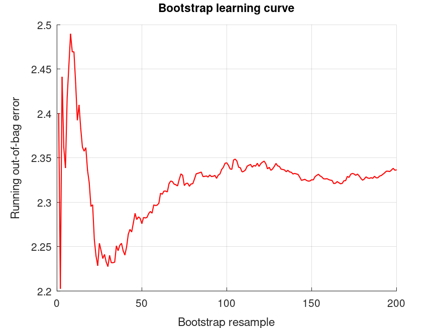
bootridge ([SAT, PPVT, Raven], MAT.X, 2, 200, .05);
% Get the output structure stored in ans from the last function call
S = ans;
Produces the following output
The bootridge function is running ...

 Empirical Bayes Ridge Regression (.632 Bootstrap Tuning) - Summary
 *******************************************************************************

 Number of predictors (p): 11

 Number of outcomes (q): 3

 Sample size: 69

 Design effect (Deff): 1

 Bootstrap resamples (nboot): 200

 Minimized .632 bootstrap prediction error: 2.07996

 Predicted R-squared: 0.307 (30.7%)

 Bootstrap optimized ridge tuning constant (lambda): 7.25059

 Effective residual degrees of freedom (df_lambda): 59.3

 Residual variances (range): [7.68, 564]

 Inferential degrees of freedom (df_t): 59.3
 Used for credible intervals and Bayes factors below.

 95% credible intervals for correlations between outcomes:
 (Prior on Fisher's z is flat/improper)

 Outcome J     Outcome I     correlation   CI_lower      CI_upper
 1             2             +0.2149       -0.04599      +0.4484
 1             3             +0.2957       +0.04040      +0.5147
 2             3             +0.2968       +0.04166      +0.5156

 95% credible intervals and Bayes factors for regression coefficients.
 Global ridge prior contribution to posterior precision: 20.77 %
 Stability selection (SS): >97.5% for the (-) or (+) sign of the coefficient.
 SS probabilities are reported in S.stability

 Outcome 1:
 coefficient   CI_lower      CI_upper      lnBF10    SS  prior
 +37.87        +31.77        +43.98        +NaN          U (-Inf, Inf)
 +6.490        -3.554        +16.53        +0.275        t (0, 8.82, 59.3)
 +1.185        -0.7453       +3.115        -0.129        t (0, 2.34, 59.3)
 +1.113        -0.4437       +2.670        +0.0729       t (0, 2.01, 59.3)
 -2.441        -3.920        -0.9626       +4.31     (-) t (0, 1.61, 59.3)
 +2.127        +0.7229       +3.531        +3.64     (+) t (0, 1.42, 59.3)
 +0.8202       -0.5386       +2.179        -0.0338       t (0, 1.46, 59.3)
 +2.592        -1.316        +6.500        -0.0302       t (0, 4.87, 59.3)
 +2.241        -0.8743       +5.356        +0.0852       t (0, 4.03, 59.3)
 -2.339        -5.306        +0.6272       +0.460        t (0, 3.23, 59.3)
 +3.362        +0.5435       +6.179        +2.05     (+) t (0, 2.87, 59.3)
 -1.699        -4.450        +1.053        -0.0223       t (0, 3.02, 59.3)

 Outcome 2:
 coefficient   CI_lower      CI_upper      lnBF10    SS  prior
 +72.38        +69.54        +75.21        +NaN          U (-Inf, Inf)
 +11.51        +6.840        +16.17        +9.81     (+) t (0, 4.10, 59.3)
 +0.2438       -0.6527       +1.140        -0.736        t (0, 1.09, 59.3)
 -0.1094       -0.8324       +0.6136       -0.903        t (0, 0.934, 59.3)
 -0.1821       -0.8689       +0.5047       -0.636        t (0, 0.748, 59.3)
 +1.126        +0.4736       +1.778        +4.82     (+) t (0, 0.658, 59.3)
 +0.5167       -0.1144       +1.148        +0.568        t (0, 0.679, 59.3)
 -0.1079       -1.923        +1.707        -0.905        t (0, 2.26, 59.3)
 +0.7991       -0.6477       +2.246        -0.335        t (0, 1.87, 59.3)
 +0.006221     -1.372        +1.384        -0.780        t (0, 1.50, 59.3)
 +0.09108      -1.218        +1.400        -0.701        t (0, 1.33, 59.3)
 +0.1488       -1.129        +1.427        -0.761        t (0, 1.40, 59.3)

 Outcome 3:
 coefficient   CI_lower      CI_upper      lnBF10    SS  prior
 +14.20        +13.48        +14.91        +NaN          U (-Inf, Inf)
 +1.049        -0.1227       +2.221        +1.03     (+) t (0, 1.03, 59.3)
 +0.1118       -0.1134       +0.3371       -0.389        t (0, 0.273, 59.3)
 +0.2157       +0.03400      +0.3973       +1.79     (+) t (0, 0.235, 59.3)
 +0.03120      -0.1414       +0.2038       -0.712        t (0, 0.188, 59.3)
 +0.02972      -0.1341       +0.1935       -0.636        t (0, 0.165, 59.3)
 -0.03604      -0.1946       +0.1225       -0.662        t (0, 0.171, 59.3)
 -0.1310       -0.5871       +0.3251       -0.745        t (0, 0.568, 59.3)
 +0.3330       -0.03056      +0.6965       +0.711    (+) t (0, 0.470, 59.3)
 -0.2740       -0.6202       +0.07219      +0.469        t (0, 0.377, 59.3)
 +0.09246      -0.2364       +0.4213       -0.551        t (0, 0.335, 59.3)
 -0.04850      -0.3696       +0.2726       -0.742        t (0, 0.353, 59.3)
and the following figure
| Figure 1 |
|---|
 |
Demonstration 2
The following code
% Simple linear regression. The data represents salaries of employees and
% their years of experience, modified from Allena Venkata. The salaries are
% in units of 1000 dollars per annum.
years = [1.20 1.40 1.60 2.10 2.30 3.00 3.10 3.30 3.30 3.80 4.00 4.10 ...
4.10 4.20 4.60 5.00 5.20 5.40 6.00 6.10 6.90 7.20 8.00 8.30 ...
8.80 9.10 9.60 9.70 10.40 10.60]';
salary = [39 46 38 44 40 57 60 54 64 57 63 56 57 57 61 68 66 83 81 94 92 ...
98 101 114 109 106 117 113 122 122]';
fprintf ('The bootridge function is running ...\n')
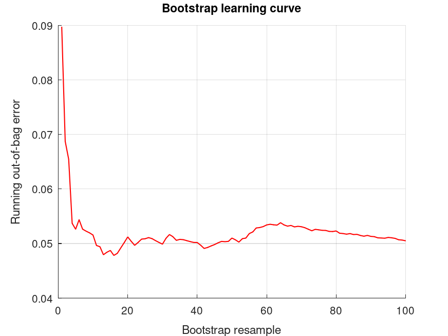
bootridge (salary, years);
% We can see from the intercept that the starting starting salary is $25.2 K
% and that salary increase per year of experience is $9.4 K.
Produces the following output
The bootridge function is running ...

 Empirical Bayes Ridge Regression (.632 Bootstrap Tuning) - Summary
 *******************************************************************************

 Number of predictors (p): 1

 Number of outcomes (q): 1

 Sample size: 30

 Design effect (Deff): 1

 Bootstrap resamples (nboot): 100

 Minimized .632 bootstrap prediction error: 0.045731

 Predicted R-squared: 0.954 (95.4%)

 Bootstrap optimized ridge tuning constant (lambda): 0.0767424

 Effective residual degrees of freedom (df_lambda): 28.0

 Residual variance (sigma^2): 32.8

 Inferential degrees of freedom (df_t): 28.0
 Used for credible intervals and Bayes factors below.

 95% credible intervals and Bayes factors for regression coefficients.
 Global ridge prior contribution to posterior precision: 0.26 %
 Stability selection (SS): >97.5% for the (-) or (+) sign of the coefficient.
 SS probabilities are reported in S.stability

 Outcome 1:
 coefficient   CI_lower      CI_upper      lnBF10    SS  prior
 +24.92        +20.25        +29.59        +NaN          U (-Inf, Inf)
 +9.430        +8.663        +10.20        +42.9     (+) t (0, 7.29, 28.0)
and the following figure
| Figure 1 |
|---|
 |
Demonstration 3
The following code
% One-way repeated measures design.
% The data is from a study on the number of words recalled by 10 subjects
% for three time condtions, in Loftus & Masson (1994) Psychon Bull Rev.
% 1(4):476-490, Table 2.
words = [10 13 13; 6 8 8; 11 14 14; 22 23 25; 16 18 20; ...
15 17 17; 1 1 4; 12 15 17; 9 12 12; 8 9 12];
seconds = [1 2 5; 1 2 5; 1 2 5; 1 2 5; 1 2 5; ...
1 2 5; 1 2 5; 1 2 5; 1 2 5; 1 2 5;];
subject = [ 1 1 1; 2 2 2; 3 3 3; 4 4 4; 5 5 5; ...
6 6 6; 7 7 7; 8 8 8; 9 9 9; 10 10 10];
% Frequentist framework: wild bootstrap of linear model, with orthogonal
% polynomial contrast coding followed up with treatment vs control
% hypothesis testing.
MAT = bootlm (words, {subject,seconds}, 'display', 'off', 'varnames', ...
{'subject','seconds'}, 'model', 'linear', 'contrasts', ...
'poly', 'dim', 2, 'posthoc', 'trt_vs_ctrl', 'nboot', 0);
% Ridge regression and bayesian analysis of posthoc comparisons
fprintf ('The bootridge function is running ...\n')
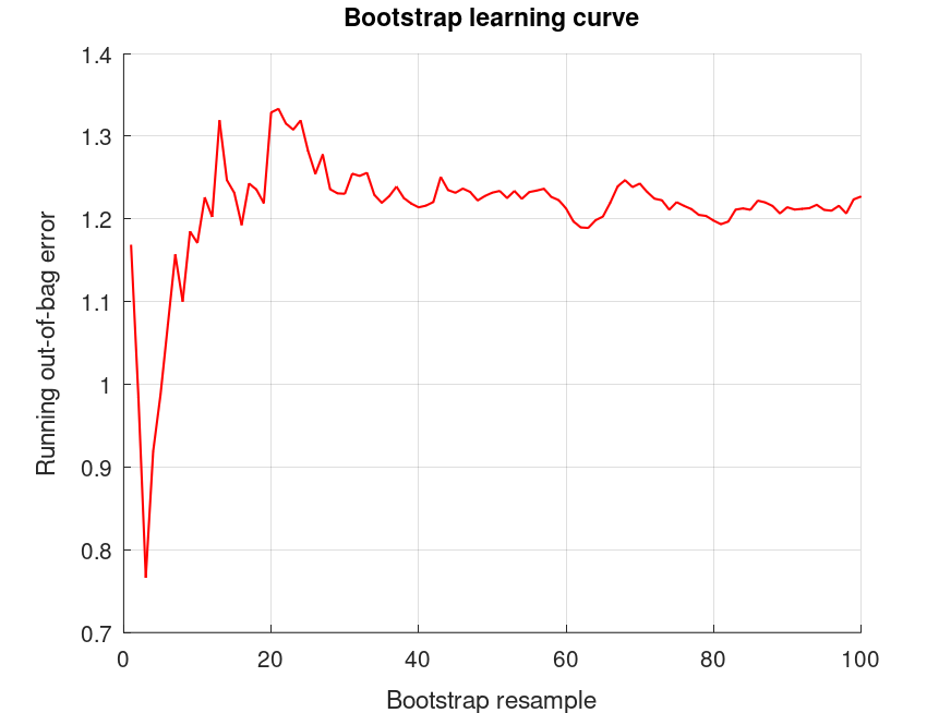
bootridge (MAT.Y, MAT.X, '*', 200, 0.05, MAT.L);
% Frequentist framework: wild bootstrap of linear model, with orthogonal
% polynomial contrast coding followed up estimating marginal means.
MAT = bootlm (words, {subject,seconds}, 'display', 'off', 'nboot', 0, ...
'model', 'linear', 'contrasts', 'poly', 'dim', 2);
% Ridge regression and bayesian analysis of model estimates. Note that group-
% mean Bayes Factors are NaN under the flat prior on the intercept whereas
% the contrasts we just calculated had proper Normal priors.
fprintf ('The bootridge function is running ...\n')
bootridge (MAT.Y, MAT.X, '*', 200, 0.05, MAT.L);
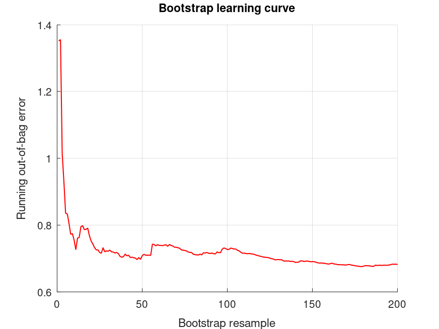
Produces the following output
The bootridge function is running ...

 Empirical Bayes Ridge Regression (.632 Bootstrap Tuning) - Summary
 *******************************************************************************

 Number of predictors (p): 11

 Number of outcomes (q): 1

 Sample size: 30

 Design effect (Deff): 1

 Bootstrap resamples (nboot): 200

 Minimized .632 bootstrap prediction error: 0.117537

 Predicted R-squared: 0.882 (88.2%)

 Bootstrap optimized ridge tuning constant (lambda): 0.028454

 Effective residual degrees of freedom (df_lambda): 18.1

 Residual variance (sigma^2): 0.616

 Inferential degrees of freedom (df_t): 18.1
 Used for credible intervals and Bayes factors below.

 95% credible intervals and Bayes factors for linear estimates.
 Global ridge prior contribution to posterior precision: 0.82 %

 Outcome 1:
 estimate      CI_lower      CI_upper      lnBF10        prior
 +1.994        +1.258        +2.731        +6.86         t (0, 6.58, 18.1)
 +3.191        +2.455        +3.927        +13.5         t (0, 6.58, 18.1)

The bootridge function is running ...

 Empirical Bayes Ridge Regression (.632 Bootstrap Tuning) - Summary
 *******************************************************************************

 Number of predictors (p): 11

 Number of outcomes (q): 1

 Sample size: 30

 Design effect (Deff): 1

 Bootstrap resamples (nboot): 200

 Minimized .632 bootstrap prediction error: 0.117537

 Predicted R-squared: 0.882 (88.2%)

 Bootstrap optimized ridge tuning constant (lambda): 0.028454

 Effective residual degrees of freedom (df_lambda): 18.1

 Residual variance (sigma^2): 0.616

 Inferential degrees of freedom (df_t): 18.1
 Used for credible intervals and Bayes factors below.

 95% credible intervals and Bayes factors for linear estimates.
 Global ridge prior contribution to posterior precision: 0.82 %

 Outcome 1:
 estimate      CI_lower      CI_upper      lnBF10        prior
 +11.00        +10.48        +11.53        +NaN          U (-Inf, Inf)
 +13.00        +12.48        +13.52        +NaN          U (-Inf, Inf)
 +14.20        +13.67        +14.72        +NaN          U (-Inf, Inf)
and the following figure
| Figure 1 |
|---|
 |
Demonstration 4
The following code
% One-way design with continuous covariate. The data is from a study of the
% additive effects of species and temperature on chirpy pulses of crickets,
% from Stitch, The Worst Stats Text eveR
pulse = [67.9 65.1 77.3 78.7 79.4 80.4 85.8 86.6 87.5 89.1 ...
98.6 100.8 99.3 101.7 44.3 47.2 47.6 49.6 50.3 51.8 ...
60 58.5 58.9 60.7 69.8 70.9 76.2 76.1 77 77.7 84.7]';
temp = [20.8 20.8 24 24 24 24 26.2 26.2 26.2 26.2 28.4 ...
29 30.4 30.4 17.2 18.3 18.3 18.3 18.9 18.9 20.4 ...
21 21 22.1 23.5 24.2 25.9 26.5 26.5 26.5 28.6]';
species = {'ex' 'ex' 'ex' 'ex' 'ex' 'ex' 'ex' 'ex' 'ex' 'ex' 'ex' ...
'ex' 'ex' 'ex' 'niv' 'niv' 'niv' 'niv' 'niv' 'niv' 'niv' ...
'niv' 'niv' 'niv' 'niv' 'niv' 'niv' 'niv' 'niv' 'niv' 'niv'};
% Estimate regression coefficients using 'anova' contrast coding
MAT = bootlm (pulse, {temp, species}, 'model', 'linear', ...
'continuous', 1, 'display', 'off', ...
'contrasts', 'anova', 'nboot', 0);
% Ridge regression and bayesian analysis of regression coefficients
% MAT.X: column 1 is intercept, column 2 is temp (continuous), column 3
% is species (categorical).
fprintf ('The bootridge function is running ...\n')
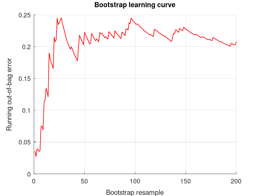
bootridge (MAT.Y, MAT.X, 3, 200, 0.05);
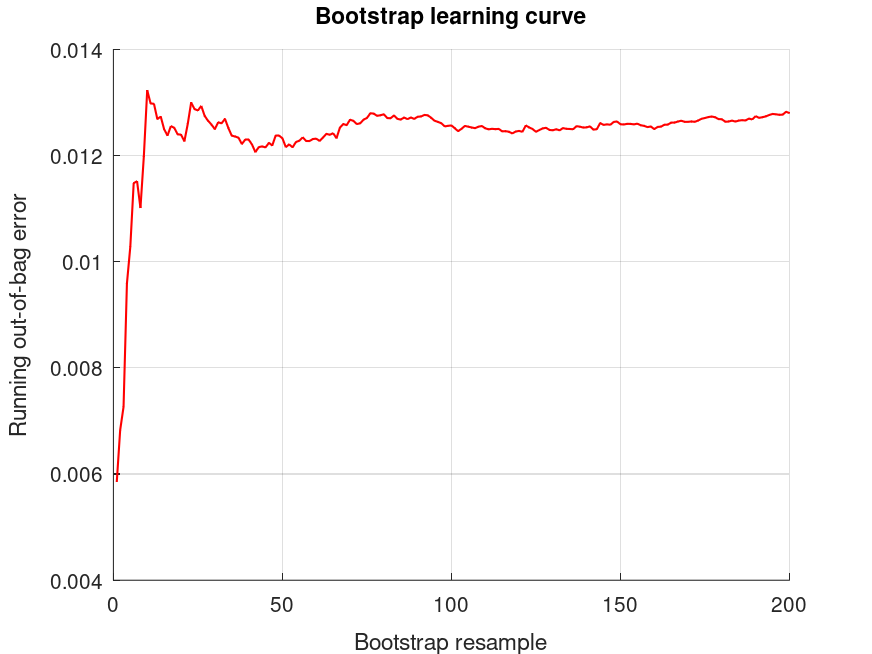
Produces the following output
The bootridge function is running ...

 Empirical Bayes Ridge Regression (.632 Bootstrap Tuning) - Summary
 *******************************************************************************

 Number of predictors (p): 2

 Number of outcomes (q): 1

 Sample size: 31

 Design effect (Deff): 1

 Bootstrap resamples (nboot): 200

 Minimized .632 bootstrap prediction error: 0.0122387

 Predicted R-squared: 0.988 (98.8%)

 Bootstrap optimized ridge tuning constant (lambda): 0.0310279

 Effective residual degrees of freedom (df_lambda): 28.0

 Residual variance (sigma^2): 3.19

 Inferential degrees of freedom (df_t): 28.0
 Used for credible intervals and Bayes factors below.

 95% credible intervals and Bayes factors for regression coefficients.
 Global ridge prior contribution to posterior precision: 0.33 %
 Stability selection (SS): >97.5% for the (-) or (+) sign of the coefficient.
 SS probabilities are reported in S.stability

 Outcome 1:
 coefficient   CI_lower      CI_upper      lnBF10    SS  prior
 +73.37        +72.71        +74.03        +NaN          U (-Inf, Inf)
 +3.601        +3.402        +3.800        +53.4     (+) t (0, 2.65, 28.0)
 -10.03        -11.53        -8.528        +26.9     (-) t (0, 10.1, 28.0)
and the following figure
| Figure 1 |
|---|
 |
Demonstration 5
The following code
 % Variations in design for two-way ANOVA (2x2) with interaction.

 % Arousal was measured in rodents assigned to four experimental groups in a
 % between-subjects design with two factors: group (lesion/control) and
 % stimulus (fearful/neutral). In this design, each rodent is allocated to one
 % combination of levels in group and stimulus, and a single measurment of
 % arousal is made. The question we are asking here is, does the effect of a
 % fear-inducing stimulus on arousal depend on whether or not rodents had a
 % lesion?

 group = {'control' 'control' 'control' 'control' 'control' 'control' ...
          'lesion'  'lesion'  'lesion'  'lesion'  'lesion'  'lesion'  ...
          'control' 'control' 'control' 'control' 'control' 'control' ...
          'lesion'  'lesion'  'lesion'  'lesion'  'lesion'  'lesion'};

 stimulus = {'fearful' 'fearful' 'fearful' 'fearful' 'fearful' 'fearful' ...
             'fearful' 'fearful' 'fearful' 'fearful' 'fearful' 'fearful' ...
             'neutral' 'neutral' 'neutral' 'neutral' 'neutral' 'neutral' ...
             'neutral' 'neutral' 'neutral' 'neutral' 'neutral' 'neutral'};

 arousal = [0.78 0.86 0.65 0.83 0.78 0.81 0.65 0.69 0.61 0.65 0.59 0.64 ...
            0.54 0.6 0.67 0.63 0.56 0.55 0.645 0.565 0.625 0.485 0.655 0.515];

 % Fit between-subjects design
 [STATS, BOOTSTAT, AOVSTAT, PRED_ERR, MAT] = bootlm (arousal, ...
                                   {group, stimulus}, 'seed', 1, ...
                                   'display', 'off', 'contrasts', 'simple', ...
                                   'model', 'full', ...
                                   'method', 'bayes');

 % Ridge regression and bayesian analysis of regression coefficients
 % MAT.X: column 1 is intercept, column 2 is temp (continuous), column 3
 % is species (categorical).
 fprintf ('The bootridge function is running ...\n')
 bootridge (MAT.Y, MAT.X, '*', 200, 0.05);

 % Now imagine the design is repeated stimulus measurements in each rodent
 ID = [1 2 3 4 5 6 7 8 9 10 11 12 1 2 3 4 5 6 7 8 9 10 11 12]';

 % Fit model including ID as a blocking-factor
 MAT = bootlm (arousal, {ID, group, stimulus}, 'seed', 1, 'nboot', 0, ...
               'display', 'off', 'contrasts', 'simple', 'method', 'bayes', ...
               'model', [1 0 0; 0 1 0; 0 0 1; 0 1 1]);

 % Ridge regression and bayesian analysis of regression coefficients
 % MAT.X: column 1 is intercept, column 2 is temp (continuous), column 3
 % is species (categorical).
 fprintf ('The bootridge function is running ...\n')
 bootridge (MAT.Y, MAT.X, '*', 200, 0.05);
Produces the following output
The bootridge function is running ...

 Empirical Bayes Ridge Regression (.632 Bootstrap Tuning) - Summary
 *******************************************************************************

 Number of predictors (p): 3

 Number of outcomes (q): 1

 Sample size: 24

 Design effect (Deff): 1

 Bootstrap resamples (nboot): 200

 Minimized .632 bootstrap prediction error: 0.41427

 Predicted R-squared: 0.586 (58.6%)

 Bootstrap optimized ridge tuning constant (lambda): 0.305249

 Effective residual degrees of freedom (df_lambda): 20.3

 Residual variance (sigma^2): 0.00356

 Inferential degrees of freedom (df_t): 20.3
 Used for credible intervals and Bayes factors below.

 95% credible intervals and Bayes factors for regression coefficients.
 Global ridge prior contribution to posterior precision: 8.86 %
 Stability selection (SS): >97.5% for the (-) or (+) sign of the coefficient.
 SS probabilities are reported in S.stability

 Outcome 1:
 coefficient   CI_lower      CI_upper      lnBF10    SS  prior
 +0.6492       +0.6238       +0.6746       +NaN          U (-Inf, Inf)
 -0.07454      -0.1241       -0.02501      +2.69     (-) t (0, 0.108, 20.3)
 -0.1189       -0.1685       -0.06942      +7.04     (-) t (0, 0.108, 20.3)
 +0.1136       +0.02100      +0.2061       +2.08     (+) t (0, 0.108, 20.3)

The bootridge function is running ...

 Empirical Bayes Ridge Regression (.632 Bootstrap Tuning) - Summary
 *******************************************************************************

 Number of predictors (p): 14

 Number of outcomes (q): 1

 Sample size: 24

 Design effect (Deff): 1

 Bootstrap resamples (nboot): 200

 Minimized .632 bootstrap prediction error: 0.541584

 Predicted R-squared: 0.458 (45.8%)

 Bootstrap optimized ridge tuning constant (lambda): 1.34378

 Effective residual degrees of freedom (df_lambda): 15.2

 Residual variance (sigma^2): 0.00422

 Inferential degrees of freedom (df_t): 15.2
 Used for credible intervals and Bayes factors below.

 95% credible intervals and Bayes factors for regression coefficients.
 Global ridge prior contribution to posterior precision: 40.29 %
 Stability selection (SS): >97.5% for the (-) or (+) sign of the coefficient.
 SS probabilities are reported in S.stability

 Outcome 1:
 coefficient   CI_lower      CI_upper      lnBF10    SS  prior
 +0.6492       +0.6209       +0.6774       +NaN          U (-Inf, Inf)
 +0.03475      -0.04703      +0.1165       +0.0470       t (0, 0.0561, 15.2)
 -0.007114     -0.08890      +0.07467      -0.359        t (0, 0.0561, 15.2)
 +0.03475      -0.04703      +0.1165       +0.0470       t (0, 0.0561, 15.2)
 -0.001133     -0.08292      +0.08065      -0.377        t (0, 0.0561, 15.2)
 +0.004848     -0.07694      +0.08663      -0.369        t (0, 0.0561, 15.2)
 +0.01436      -0.06856      +0.09729      -0.292        t (0, 0.0561, 15.2)
 +0.002400     -0.08053      +0.08533      -0.362        t (0, 0.0561, 15.2)
 -0.003582     -0.08651      +0.07934      -0.359        t (0, 0.0561, 15.2)
 -0.03349      -0.1164       +0.04944      +0.0206       t (0, 0.0561, 15.2)
 -0.0005911    -0.08352      +0.08233      -0.364        t (0, 0.0561, 15.2)
 -0.02751      -0.1104       +0.05542      -0.102        t (0, 0.0561, 15.2)
 -0.04841      -0.1174       +0.02057      +0.562    (-) t (0, 0.0561, 15.2)
 -0.1021       -0.1532       -0.05109      +5.52     (-) t (0, 0.0561, 15.2)
 +0.07209      -0.009930     +0.1541       +1.30     (+) t (0, 0.0561, 15.2)
and the following figure
| Figure 1 |
|---|
 |
Demonstration 6
The following code
 % Analysis of nested one-way design.

 % Nested model example from:
 % https://www.southampton.ac.uk/~cpd/anovas/datasets/#Chapter2

 data = [4.5924 7.3809 21.322; -0.5488 9.2085 25.0426; ...
         6.1605 13.1147 22.66; 2.3374 15.2654 24.1283; ...
         5.1873 12.4188 16.5927; 3.3579 14.3951 10.2129; ...
         6.3092 8.5986 9.8934; 3.2831 3.4945 10.0203];

 clustid = [1 3 5; 1 3 5; 1 3 5; 1 3 5; ...
            2 4 6; 2 4 6; 2 4 6; 2 4 6];

 group = {'A' 'B' 'C'; 'A' 'B' 'C'; 'A' 'B' 'C'; 'A' 'B' 'C'; ...
          'A' 'B' 'C'; 'A' 'B' 'C'; 'A' 'B' 'C'; 'A' 'B' 'C'};

 % Fit model with cluster-based resampling. We are using Bayesian bootstrap
 % using 'auto' prior, which effectively applies Bessel's correction to the
 % variance of the bootstrap distribution for the contrasts (trt_vs_ctrl).
 % Use 'treatment' coding and return regression coefficients since our
 % intention is to use the posterior distributions from bayesian bootstrap
 % to calculate the design effect.
 [STATS, BOOTSTAT, AOVSTAT, PREDERR, MAT] = bootlm (data, {group}, ...
      'clustid', clustid, 'seed', 1, 'display', 'off', 'contrasts', ...
      'treatment', 'method', 'bayes', 'prior', 'auto');

 % Or we can get a obtain the design effect empirically using resampling.
 % We already fit the model accounting for clustering, now lets fit it
 % under I.I.D. (i.e. without clustering). As above, use 'treatment' coding.
 [STATS_SRS, BOOTSTAT_SRS] = bootlm (data, {group}, 'seed', 1, 'display', ...
      'off', 'contrasts', 'treatment', 'method', 'bayes');

 % Empirically calculate the design effect averaged over the variance of
 % of the contrasts we are interested in
 Var_true = var (BOOTSTAT, 0, 2);
 Var_iid  = var (BOOTSTAT_SRS, 0, 2);
 DEFF = mean (Var_true ./ Var_iid);
 % Or more simply, we can use the deffcalc function, which does the same thing.
 % We take the mean DEFF across all contrasts for a stable global penalty.
 DEFF = mean (deffcalc (BOOTSTAT, BOOTSTAT_SRS))

 % Refit the model using orthogonal (helmert) contrasts and a hypothesis
 % matrix specifying pairwise comparisons. Set nboot to 0 to avoid resampling.
 MAT = bootlm (data, {group}, 'clustid', clustid, 'display', 'off', ...
               'contrasts', 'helmert', 'dim', 1, 'posthoc', 'pairwise', ...
               'nboot', 0);

 % Fit a cluster-robust empirical Bayes model using our bootstrap estimate of
 % the design effect and using the hypothesis matrix to define the comparisons
 fprintf ('The bootridge function is running ...\n')
 bootridge (MAT.Y, MAT.X, '*', 200, 0.05, MAT.L, DEFF);

 % Compare this to using a maximum cluster size as an upperbound for Deff
 g = max (accumarray (clustid(:), 1, [], @sum));  % g is max. cluster size
 fprintf ('The bootridge function is running ...\n')
 bootridge (MAT.Y, MAT.X, '*', 200, 0.05, MAT.L, g); % Upperbound DEFF is g

 % Note: Using the empirical DEFF (~1.5) instead of the upper-bound (4.0)
 % recovers inferential power, as seen by the higher Bayes Factor (lnBF10)
 % and narrower credible intervals.
Produces the following output
DEFF = 1.4556
The bootridge function is running ...

 Empirical Bayes Ridge Regression (.632 Bootstrap Tuning) - Summary
 *******************************************************************************

 Number of predictors (p): 2

 Number of outcomes (q): 1

 Sample size: 24

 Design effect (Deff): 1.46

 Bootstrap resamples (nboot): 200

 Minimized .632 bootstrap prediction error: 0.463286

 Predicted R-squared: 0.537 (53.7%)

 Bootstrap optimized ridge tuning constant (lambda, Deff-adjusted): 0.318356

 Effective residual degrees of freedom (df_lambda): 21.1

 Residual variance (sigma^2, Deff-inflated): 31.8

 Inferential degrees of freedom (df_t, Deff-adjusted): 13.6
 Used for credible intervals and Bayes factors below.

 95% credible intervals and Bayes factors for linear estimates.
 Global ridge prior contribution to posterior precision: 6.50 %

 Outcome 1:
 estimate      CI_lower      CI_upper      lnBF10        prior
 -6.336        -12.21        -0.4634       +1.03         t (0, 11.2, 13.6)
 -12.82        -18.69        -6.947        +5.63         t (0, 11.2, 13.6)
 -6.483        -12.32        -0.6518       +1.26         t (0, 9.99, 13.6)

The bootridge function is running ...

 Empirical Bayes Ridge Regression (.632 Bootstrap Tuning) - Summary
 *******************************************************************************

 Number of predictors (p): 2

 Number of outcomes (q): 1

 Sample size: 24

 Design effect (Deff): 4

 Bootstrap resamples (nboot): 200

 Minimized .632 bootstrap prediction error: 0.463286

 Predicted R-squared: 0.537 (53.7%)

 Bootstrap optimized ridge tuning constant (lambda, Deff-adjusted): 0.115848

 Effective residual degrees of freedom (df_lambda): 21.0

 Residual variance (sigma^2, Deff-inflated): 87.1

 Inferential degrees of freedom (df_t, Deff-adjusted): 3.05
 Used for credible intervals and Bayes factors below.

 95% credible intervals and Bayes factors for linear estimates.
 Global ridge prior contribution to posterior precision: 2.47 %

 Outcome 1:
 estimate      CI_lower      CI_upper      lnBF10        prior
 -6.532        -21.08        +8.017        -0.871        t (0, 30.7, 3.05)
 -13.33        -27.88        +1.214        +0.776        t (0, 30.7, 3.05)
 -6.802        -21.31        +7.708        -0.691        t (0, 27.4, 3.05)
and the following figure
| Figure 1 |
|---|
 |
Demonstration 7
The following code
 %% --- Stress-test: Simulated Large-Scale Patch-seq Project (bootridge) ---
 %% N = 7500 cells
 %% p = 15 features
 %% q = 2000 genes
 %% This tests memory handling and global lambda optimization.

 N = 7500;
 p = 15;
 q = 2000;
 nboot = 100;

 % Set random seeds for the simulation
 rand ('seed', 123);
 randn ('seed', 123);

 fprintf ('Simulate Large-Scale Patch-seq Dataset (%d x %d)...\n', N, q);

 % Generate design matrix X (E-phys features)
 X = [ones(N,1), randn(N, p-1)];

 % Generate sparse multivariate outcome Y (Gene expression)
 % Approx 120MB of data
 true_beta = randn (p, q) .* (rand (p, q) > 0.9);

 % Set signal-to-noise ratio to 0.5
 target_snr = 0.5;
 beta_no_intercept = true_beta(2:end, :);
 signal_var_per_gene = sum (beta_no_intercept.^2, 1);
 snr_per_gene = signal_var_per_gene / (0.5^2);
 current_snr = mean (snr_per_gene);
 scale = sqrt (target_snr / current_snr);
 true_beta(2:end, :) = true_beta(2:end, :) * scale;

 % Introduce correlations
 n_factors = 10; % 10 latent biological processes
 latent_X = randn (N, n_factors);
 % Each latent factor affects about 10% of genes (sparse correlation)
 latent_beta = randn (n_factors, q) .* (rand (n_factors, q) > 0.90);

 % Simulate the data with added correlated noise (0.2 strength)
 Y = X * true_beta + (latent_X * latent_beta * 0.2) + randn (N, q) * 0.5;

 fprintf('Running bootridge ...\n');
 tic;
 % Use TOL = 0.05 for faster convergence in demo
 S = bootridge (Y, X, [], nboot, 0.05, [], 1, 123, 0.05);
 runtime = toc;

 fprintf ('\n--- Performance Results ---\n');
 fprintf ('Runtime: %.2f seconds\n', runtime);
 fprintf ('Optimized Lambda: %.6f\n', S.lambda);
 fprintf ('Total Iterations: %d\n', S.iter);

 % Accuracy Check on a random gene
 target_gene = ceil (rand * q);
 estimated = S.coefficient(:, target_gene);
 actual = true_beta(:, target_gene);
 correlation = corr (estimated, actual);

 % ROC statistics
 threshold = 3;                                    % corresponds to BF10 of 20
 fp = sum (S.lnBF10(true_beta == 0) >  threshold); % false positives
 tp = sum (S.lnBF10(true_beta ~= 0) >  threshold); % true positives
 fn = sum (S.lnBF10(true_beta ~= 0) <= threshold); % missed true effects
 power      = tp / (tp + fn);                      % true positive rate
 fp_rate    = fp / sum (true_beta(:) == 0);        % false positive rate
 precision  = tp / (tp + fp);                      % true discovery rate

 fprintf ('Correlation of estimates for Gene %d: %.4f\n', ...
          target_gene, correlation);
 fprintf ('Number of coefficients: [%s] (Expected: [15 x 2000])\n', ...
           num2str (size (S.coefficient)));
 fprintf ('Number of pairwise correlations: [%s] (Expected: 1999000)\n', ...
           num2str (size (S.RTAB, 1)));
 fprintf ('Positive detections (i.e. discoveries) defined hereon as BF10 > 20');
 fprintf ('\nFalse positive rate (FPR): %.1f%%\n', fp_rate * 100);
 fprintf ('Precision (i.e. 1-FDR): %.1f%%\n', precision * 100);
 fprintf ('Power (i.e. TPR): %.1f%%\n', power * 100);
Produces the following output
Simulate Large-Scale Patch-seq Dataset (7500 x 2000)...
Running bootridge ...

--- Performance Results ---
Runtime: 893.60 seconds
Optimized Lambda: 65.132264
Total Iterations: 12
Correlation of estimates for Gene 158: 0.9952
Number of coefficients: [15  2000] (Expected: [15 x 2000])
Number of pairwise correlations: [1999000] (Expected: 1999000)
Positive detections (i.e. discoveries) defined hereon as BF10 > 20
False positive rate (FPR): 0.1%
Precision (i.e. 1-FDR): 98.9%
Power (i.e. TPR): 94.8%
Demonstration 8
The following code
 %% --- Stress-test: Large-Scale Differential Gene Expression (DGE) Simulation ---
 %% Scenario: Bulk RNA-seq Case-Control Study (e.g., Disease vs. Healthy)
 %% N = 300 samples (e.g., 150 Patient / 150 Control)
 %% p = 50 covariates (e.g., 1 Group Indicator + 49 Technical/PEER factors)
 %% q = 15000 genes (Simultaneously modeled outcomes)
 %%
 %% This demo evaluates the multivariate efficiency of bootridge across
 %% the typical protein-coding transcriptome size, testing memory handling
 %% and the speed of global lambda optimization.

 % 1. Setup Dimensions
 N = 300;      % Total biological samples (Bulk RNA-seq)
 p = 50;       % 1 Experimental Group + technical covariates (Age, RIN, Batch)
 q = 15000;    % Total Genes analyzed in this "chunk"
 nboot = 100;  % Number of bootstrap resamples
 % Set random seeds for the simulation
 rand ('seed', 123);
 randn ('seed', 123);

 fprintf (cat (2, 'Simulating DGE Dataset: %d samples, %d genes, %d ', ...
                  'covariates...\n'), N, q, p);

 % 2. Generate Design Matrix X
 % Column 1: Intercept
 % Column 2: Group Indicator (0 = Control, 1 = Case)
 % Columns 3-p: Random technical noise (Covariates/PEER factors)
 Group = [zeros(N/2, 1); ones(N/2, 1)];
 Covariates = randn (N, p-2);
 X = [ones(N, 1), Group, Covariates];

 % 3. Define Biological Signal (The "True" Log-Fold Changes)
 % We simulate a realistic DGE profile:
 % 10% of genes are differentially expressed (hits).
 true_beta = zeros (p, q);
 sig_genes = ceil (rand (1, round (q * 0.10)) * q);
 true_beta(2, sig_genes) = (randn (1, length (sig_genes)) * 2); % Group effect

 % 4. Generate Expression Matrix Y (Log2 TPM / Counts)
 % Baseline + Group Effect + Gaussian noise.
 Baseline = 5 + randn (1, q);
 Y = repmat (Baseline, N, 1) + X * true_beta + randn (N, q) * 1.2;

 fprintf ('Running Multivariate bootridge (Shrinkage shared across genes)...\n');

 tic;
 % CATEGOR = 2: Treats the Group column as categorical (no variance scaling).
 % SEED = 123: Ensures reproducible bootstrap sampling.
 % TOL = 0.05: Convergence tolerance for the golden section search.
 S = bootridge (Y, X, 2, nboot, 0.05, [], 1, 123, 0.05);
 runtime = toc;

 % 5. Display Performance Results
 fprintf ('\n--- Performance Results ---\n');
 fprintf ('Runtime: %.2f seconds\n', runtime);
 fprintf ('Optimized Lambda: %.6f\n', S.lambda);

 % 6. Accuracy Check
 % Compare estimated Beta (Group Effect) against the Ground Truth Fold-Changes
 estimated_fc = S.coefficient(2, :);
 true_fc = true_beta(2, :);
 correlation = corr (estimated_fc', true_fc');

 fprintf ('Correlation of Fold-Changes across %d genes: %.4f\n', ...
          q, correlation);
 fprintf ('Number of coefficients: [%s] (Expected: [50 x 15000])\n', ...
           num2str (size (S.coefficient)));
 fprintf ('Number of pairwise correlations: [%s] (Expected: 112492500)\n', ...
           num2str (size (S.RTAB, 1)));
Produces the following output
Simulating DGE Dataset: 300 samples, 15000 genes, 50 covariates...
Running Multivariate bootridge (Shrinkage shared across genes)...

--- Performance Results ---
Runtime: 483.80 seconds
Optimized Lambda: 510.212731
Correlation of Fold-Changes across 15000 genes: 0.9759
Number of coefficients: [50  15000] (Expected: [50 x 15000])
Number of pairwise correlations: [112492500] (Expected: 112492500)
Demonstration 9
The following code
 %% --- Stress-test: High-p Voxel-wise Neural Encoding Simulation ---
 %% Scenario: Reconstructing Visual Stimuli from fMRI BOLD signals
 %% N = 500 volumes (samples), p = 8000 voxels, q = 1 stimulus feature
 %% This demo requires the signal package in octave

 % 1. Setup Dimensions
 N = 500; p = 8000; q = 1; nboot = 200;
 rand ('seed', 123); randn ('seed', 123);
 fprintf('Simulating fMRI Encoding: %d timepoints, %d voxels...\n', N, p);

 % 2. Generate Design Matrix X (The Voxels)
 %    Spatial correlation between voxels (columns) and time points (rows)
 X_raw = randn (N, p-1);
 X = [ones(N, 1), filter([0.5 1 0.5], 1, X_raw, [], 2)];
 X(:,2:end) = filter ([0.1, 0.4, 0.9, 1, 0.6, 0.2], 1, X(:,2:end), [], 1);

 % 3. Define the "Neural Code" (True Weights)
 true_beta_sparse = zeros (p, q);                       % Initialise
 active_voxels = 1 + ceil (rand (1, 25) * (p - 1));     % 50 spatial clusters
 true_beta_sparse(active_voxels) = randn (25, 1) * 100; % Active voxels
 kernel = [0.05 0.1 0.4 0.8 1 0.8 0.4 0.1 0.05];        % Smoothing kernel
 true_beta = filter (kernel, 1, true_beta_sparse);      % Smooth active voxels

 % 4. Generate outcome Y (The Stimulus)
 % Signal from smoothed clusters + Gaussian noise
 Y = X * true_beta + randn (N, q);

 % 5. Estimate Design Effect (Deff) to account for serial dependence
 % We use the autocorrelation of Y to estimate the variance inflation factor
 %
 %  Bayley, G. V., & Hammersley, J. M. (1946). The "Effective" Number of
 %    Independent Observations in an Autocorrelated Time Series. Supplement to
 %    the Journal of the Royal Statistical Society, 8(2), 184–197.
 %    https://doi.org/10.2307/2983560
 try
   info = ver;
   isoctave = any (ismember ({info.Name}, 'Octave'));
   if (isoctave)
     pkg load signal;
   end
   [r, lags] = xcov (Y - mean (Y), 10, 'coeff');
   Deff = 1 + 2 * sum (r(lags > 0));
   fprintf ('Estimated Design Effect (Deff): %.3f\n', Deff);
 catch
   Deff = 1;
 end

 % 6. Run bootridge
 fprintf ('Running bootridge (Global Lambda Optimization)...\n');
 tic;
 % Run the bootridge function
 S = bootridge (Y, X, [], nboot, 0.05, [], Deff, 123, 0.05);
 runtime = toc;

 % 7. Performance Results
 estimated_beta = S.coefficient;
 correlation = corr (estimated_beta, true_beta);
 fprintf ('\n--- Performance Results ---\n');
 fprintf ('Runtime: %.2f seconds\n', runtime);
 fprintf ('Optimized Lambda: %.6f\n', S.lambda);

 fprintf ('Correlation of Voxel Weight Map: %.4f\n', correlation);
 fprintf ('Number of coefficients: [%s] (Expected: [8000 x 1])\n', ...
           num2str (size (S.coefficient)));
Produces the following output
Simulating fMRI Encoding: 500 timepoints, 8000 voxels...
Estimated Design Effect (Deff): 3.489
Running bootridge (Global Lambda Optimization)...
Note: t-statistics evaluated with effective degrees of freedom clamped at 1 degree of freedom.

--- Performance Results ---
Runtime: 1713.78 seconds
Optimized Lambda: 0.326447
Correlation of Voxel Weight Map: 0.3970
Number of coefficients: [8000     1] (Expected: [8000 x 1])
Demonstration 10
The following code
 %  Error Control: Global Ridge vs Per-Outcome Wild Bootstrap (n = 40)
 %                  under global multicollinearity (r = 0.2)
 %
 %  --- Parameters ---
 %  n_sims   = 30;
 %  alpha    = 0.05;
 %  n_vals   = 40;
 %  p_vals   = [3, 10, 30];
 %  q_vals   = [1, 5, 10];
 %  snr_vals = [0.1, 0.2, 0.4, 0.8];
 %  seed     = 42;
 %  randn('seed', seed);
 %
 %  for p = p_vals
 %    for q = q_vals
 %      for snr = snr_vals
 %        % Accumulators
 %        fpr_r_ci = 0; fpr_r_bf = 0; fpr_r_ss = 0;
 %        fpr_w_std = 0; fpr_w_max = 0;
 %        fdr_r_ci = 0; fdr_r_bf = 0; fdr_r_ss = 0;
 %        fdr_w_std = 0; fdr_w_max = 0;
 %        pow_r_ci = 0; pow_r_bf = 0; pow_r_ss = 0;
 %        pow_w_std = 0; pow_w_max = 0;
 %        sig_hits_r = 0; type_s_r = 0; type_m_r = 0;
 %        sig_hits_w = 0; type_s_w = 0; type_m_w = 0;
 %        mse_r = 0; mse_w = 0;
 %
 %        for s = 1:n_sims
 %          % 1. Induce Predictor Correlation (r = 0.2)
 %          X_raw = randn(n_vals, p);
 %          X = bsxfun(@plus, X_raw * 0.8944, randn(n_vals, 1) * 0.4472);
 %          X = [ones(n_vals, 1), X];
 %
 %          % 2. Setup Signal (Variable 2 is the only true signal)
 %          beta_true = zeros(p+1, q);
 %          beta_true(2, :) = snr;
 %
 %          % 3. Induce Outcome Noise Correlation (r = 0.2)
 %          noise_unique = randn(n_vals, q);
 %          noise_common = randn(n_vals, 1);
 %          E = bsxfun(@plus, noise_unique * 0.8944, noise_common * 0.4472);
 %
 %          % 4. Generate Y
 %          y_raw = X * beta_true + E;
 %          y = (y_raw - mean(y_raw)) ./ std(y_raw);
 %
 %          S_r = bootridge(y, X, [], 200, alpha, [], 1, s);
 %
 %          rej_w_std = false(p+1, q);
 %          rej_w_max = false(p+1, q);
 %          coeffs_w  = zeros(p+1, q);
 %          for j = 1:q
 %            res_std = bootwild(y(:,j), X, [], 1999, alpha, s, 0);
 %            res_max = bootwild(y(:,j), X, [], 1999, {alpha}, s, 1);
 %            rej_w_std(:, j) = (res_std.pval <= alpha);
 %            rej_w_max(:, j) = (res_max.pval <= alpha);
 %            coeffs_w(:, j)  = res_max.original;
 %          end
 %
 %          % --- Indices ---
 %          null_idx = 3:(p+1);
 %          sig_idx  = 2;
 %
 %          % --- Ridge Decisions ---
 %          dec_r_ci = (S_r.CI_lower > 0 | S_r.CI_upper < 0);
 %          dec_r_bf = (S_r.lnBF10 >= 1);
 %          dec_r_ss = (S_r.stability > (1 - alpha/2));
 %
 %          % --- FDR Calculation ---
 %          fd = sum(sum(dec_r_ci(null_idx, :)));
 %          td = sum(sum(dec_r_ci(2:(p+1), :)));
 %          if td > 0, fdr_r_ci = fdr_r_ci + (fd/td); end
 %
 %          fd = sum(sum(dec_r_bf(null_idx, :)));
 %          td = sum(sum(dec_r_bf(2:(p+1), :)));
 %          if td > 0, fdr_r_bf = fdr_r_bf + (fd/td); end
 %
 %          fd = sum(sum(dec_r_ss(null_idx, :)));
 %          td = sum(sum(dec_r_ss(2:(p+1), :)));
 %          if td > 0, fdr_r_ss = fdr_r_ss + (fd/td); end
 %
 %          fd = sum(sum(rej_w_std(null_idx, :)));
 %          td = sum(sum(rej_w_std(2:(p+1), :)));
 %          if td > 0, fdr_w_std = fdr_w_std + (fd/td); end
 %
 %          fd = sum(sum(rej_w_max(null_idx, :)));
 %          td = sum(sum(rej_w_max(2:(p+1), :)));
 %          if td > 0, fdr_w_max = fdr_w_max + (fd/td); end
 %
 %          % --- FPR ---
 %          num_null_total = length(null_idx) * q;
 %          fpr_r_ci  = fpr_r_ci + (sum(sum(dec_r_ci(null_idx, :))) / ...
 %                                  num_null_total);
 %          fpr_r_bf  = fpr_r_bf + (sum(sum(dec_r_bf(null_idx, :))) / ...
 %                                  num_null_total);
 %          fpr_r_ss  = fpr_r_ss + (sum(sum(dec_r_ss(null_idx, :))) / ...
 %                                  num_null_total);
 %          fpr_w_std = fpr_w_std + (sum(sum(rej_w_std(null_idx, :))) / ...
 %                                   num_null_total);
 %          fpr_w_max = fpr_w_max + (sum(sum(rej_w_max(null_idx, :))) / ...
 %                                   num_null_total);
 %
 %          % --- Signal Analysis ---
 %          pow_r_ci  = pow_r_ci + (sum(dec_r_ci(sig_idx, :)) / q);
 %          pow_r_bf  = pow_r_bf + (sum(dec_r_bf(sig_idx, :)) / q);
 %          pow_r_ss  = pow_r_ss + (sum(dec_r_ss(sig_idx, :)) / q);
 %          pow_w_std = pow_w_std + (sum(rej_w_std(sig_idx, :)) / q);
 %          pow_w_max = pow_w_max + (sum(rej_w_max(sig_idx, :)) / q);
 %
 %          for j = 1:q
 %            if dec_r_ci(sig_idx, j)
 %              sig_hits_r = sig_hits_r + 1;
 %              if sign(S_r.coefficient(2,j)) ~= sign(snr)
 %                type_s_r = type_s_r + 1;
 %              end
 %              type_m_r = type_m_r + (abs(S_r.coefficient(2,j)) / abs(snr));
 %            end
 %            if rej_w_max(sig_idx, j)
 %              sig_hits_w = sig_hits_w + 1;
 %              if sign(coeffs_w(2,j)) ~= sign(snr)
 %                type_s_w = type_s_w + 1;
 %              end
 %              type_m_w = type_m_w + (abs(coeffs_w(2,j)) / abs(snr));
 %            end
 %          end
 %
 %          X_test = [ones(50, 1), randn(50, p)];
 %          y_test_raw = X_test * beta_true + randn(50, q);
 %          y_test = (y_test_raw - mean(y_test_raw)) ./ std(y_test_raw);
 %          mse_r = mse_r + mean(mean((y_test - X_test*S_r.coefficient).^2));
 %          mse_w = mse_w + mean(mean((y_test - X_test*coeffs_w).^2));
 %        end
 %
 %      end
 %    end
 %  end

 %
 %              |     |--- MSE ---|
 %  Cond (p,q)  | SNR |Ridge Wild
 %  ------------------------------|
 %  p3 q1       | 0.1 |1.00  1.07 |
 %  p3 q1       | 0.2 |0.98  1.04 |
 %  p3 q1       | 0.4 |0.90  0.91 |
 %  p3 q1       | 0.8 |0.68  0.69 |
 %  ------------------------------|
 %  p3 q5       | 0.1 |0.99  1.06 |
 %  p3 q5       | 0.2 |0.97  1.03 |
 %  p3 q5       | 0.4 |0.90  0.94 |
 %  p3 q5       | 0.8 |0.68  0.70 |
 %  ------------------------------|
 %  p3 q10      | 0.1 |0.99  1.07 |
 %  p3 q10      | 0.2 |0.97  1.03 |
 %  p3 q10      | 0.4 |0.90  0.94 |
 %  p3 q10      | 0.8 |0.66  0.67 |
 %  ------------------------------|
 %  p10 q1      | 0.1 |1.01  1.38 |
 %  p10 q1      | 0.2 |1.02  1.39 |
 %  p10 q1      | 0.4 |0.98  1.24 |
 %  p10 q1      | 0.8 |0.77  0.85 |
 %  ------------------------------|
 %  p10 q5      | 0.1 |1.00  1.37 |
 %  p10 q5      | 0.2 |0.99  1.35 |
 %  p10 q5      | 0.4 |0.94  1.21 |
 %  p10 q5      | 0.8 |0.75  0.88 |
 %  ------------------------------|
 %  p10 q10     | 0.1 |1.00  1.42 |
 %  p10 q10     | 0.2 |0.99  1.36 |
 %  p10 q10     | 0.4 |0.95  1.25 |
 %  p10 q10     | 0.8 |0.74  0.87 |
 %  ------------------------------|
 %  p30 q1      | 0.1 |1.13  5.49 |
 %  p30 q1      | 0.2 |1.07  5.02 |
 %  p30 q1      | 0.4 |1.05  4.51 |
 %  p30 q1      | 0.8 |0.94  3.20 |
 %  ------------------------------|
 %  p30 q5      | 0.1 |1.07  5.36 |
 %  p30 q5      | 0.2 |1.04  5.34 |
 %  p30 q5      | 0.4 |1.04  4.39 |
 %  p30 q5      | 0.8 |0.90  3.58 |
 %  ------------------------------|
 %  p30 q10     | 0.1 |1.04  5.95 |
 %  p30 q10     | 0.2 |1.05  5.71 |
 %  p30 q10     | 0.4 |1.02  4.86 |
 %  p30 q10     | 0.8 |0.87  3.18 |
 %  ------------------------------|

 %              |     |--- Ridge Pow --- |  Wild Pow   |
 %  Cond (p,q)  | SNR |CI    BF    SS    | Std   MaxT  |
 %  ---------------------------------------------------|
 %  p3 q1       | 0.1 |0.10  0.13  0.17  | 0.13  0.07  |
 %  p3 q1       | 0.2 |0.07  0.10  0.20  | 0.20  0.10  |
 %  p3 q1       | 0.4 |0.30  0.40  0.60  | 0.47  0.23  |
 %  p3 q1       | 0.8 |0.97  1.00  1.00  | 1.00  0.90  |
 %  ---------------------------------------------------|
 %  p3 q5       | 0.1 |0.00  0.01  0.09  | 0.09  0.01  |
 %  p3 q5       | 0.2 |0.10  0.15  0.32  | 0.23  0.12  |
 %  p3 q5       | 0.4 |0.39  0.57  0.70  | 0.61  0.35  |
 %  p3 q5       | 0.8 |1.00  1.00  1.00  | 0.99  0.97  |
 %  ---------------------------------------------------|
 %  p3 q10      | 0.1 |0.02  0.07  0.12  | 0.10  0.05  |
 %  p3 q10      | 0.2 |0.08  0.15  0.29  | 0.23  0.10  |
 %  p3 q10      | 0.4 |0.50  0.62  0.68  | 0.64  0.49  |
 %  p3 q10      | 0.8 |0.95  0.97  0.97  | 0.95  0.89  |
 %  ---------------------------------------------------|
 %  p10 q1      | 0.1 |0.03  0.07  0.20  | 0.13  0.00  |
 %  p10 q1      | 0.2 |0.03  0.03  0.17  | 0.07  0.03  |
 %  p10 q1      | 0.4 |0.23  0.43  0.53  | 0.43  0.13  |
 %  p10 q1      | 0.8 |0.90  0.97  1.00  | 0.97  0.83  |
 %  ---------------------------------------------------|
 %  p10 q5      | 0.1 |0.02  0.05  0.14  | 0.10  0.01  |
 %  p10 q5      | 0.2 |0.02  0.07  0.28  | 0.19  0.05  |
 %  p10 q5      | 0.4 |0.29  0.50  0.65  | 0.47  0.23  |
 %  p10 q5      | 0.8 |0.94  0.97  0.99  | 0.97  0.82  |
 %  ---------------------------------------------------|
 %  p10 q10     | 0.1 |0.00  0.00  0.09  | 0.07  0.00  |
 %  p10 q10     | 0.2 |0.01  0.06  0.24  | 0.15  0.02  |
 %  p10 q10     | 0.4 |0.29  0.46  0.71  | 0.51  0.23  |
 %  p10 q10     | 0.8 |0.94  0.98  0.99  | 0.96  0.79  |
 %  ---------------------------------------------------|
 %  p30 q1      | 0.1 |0.00  0.00  0.10  | 0.00  0.00  |
 %  p30 q1      | 0.2 |0.00  0.03  0.17  | 0.13  0.03  |
 %  p30 q1      | 0.4 |0.17  0.30  0.67  | 0.17  0.03  |
 %  p30 q1      | 0.8 |0.83  0.90  1.00  | 0.57  0.10  |
 %  ---------------------------------------------------|
 %  p30 q5      | 0.1 |0.01  0.02  0.15  | 0.11  0.02  |
 %  p30 q5      | 0.2 |0.00  0.01  0.23  | 0.09  0.01  |
 %  p30 q5      | 0.4 |0.13  0.33  0.71  | 0.25  0.07  |
 %  p30 q5      | 0.8 |0.71  0.87  0.98  | 0.45  0.17  |
 %  ---------------------------------------------------|
 %  p30 q10     | 0.1 |0.00  0.00  0.15  | 0.11  0.01  |
 %  p30 q10     | 0.2 |0.01  0.06  0.27  | 0.11  0.01  |
 %  p30 q10     | 0.4 |0.05  0.22  0.57  | 0.17  0.02  |
 %  p30 q10     | 0.8 |0.74  0.89  0.97  | 0.54  0.15  |
 %  ---------------------------------------------------|

 %              |     |Ridge Errors  | Wild Errors   |
 %  Cond (p,q)  | SNR |TypeS  TypeM  | TypeS  TypeM  |
 %  -------------------------------------------------|
 %  p3 q1       | 0.1 |0.333  3.53   | 0.500  4.89   |
 %  p3 q1       | 0.2 |0.000  2.02   | 0.000  2.47   |
 %  p3 q1       | 0.4 |0.000  0.86   | 0.000  1.17   |
 %  p3 q1       | 0.8 |0.000  0.66   | 0.000  0.79   |
 %  -------------------------------------------------|
 %  p3 q5       | 0.1 |0.000   ND    | 0.000  3.42   |
 %  p3 q5       | 0.2 |0.000  1.29   | 0.000  2.15   |
 %  p3 q5       | 0.4 |0.000  0.80   | 0.000  1.23   |
 %  p3 q5       | 0.8 |0.000  0.70   | 0.000  0.81   |
 %  -------------------------------------------------|
 %  p3 q10      | 0.1 |0.000  2.55   | 0.067  4.27   |
 %  p3 q10      | 0.2 |0.000  1.33   | 0.000  2.46   |
 %  p3 q10      | 0.4 |0.000  0.82   | 0.000  1.19   |
 %  p3 q10      | 0.8 |0.000  0.67   | 0.000  0.81   |
 %  -------------------------------------------------|
 %  p10 q1      | 0.1 |0.000  1.90   | 0.000  0.00   |
 %  p10 q1      | 0.2 |0.000  1.49   | 0.000  2.51   |
 %  p10 q1      | 0.4 |0.000  0.84   | 0.000  1.47   |
 %  p10 q1      | 0.8 |0.000  0.54   | 0.000  0.82   |
 %  -------------------------------------------------|
 %  p10 q5      | 0.1 |0.000  2.36   | 0.000  6.21   |
 %  p10 q5      | 0.2 |0.000  1.10   | 0.000  2.83   |
 %  p10 q5      | 0.4 |0.000  0.65   | 0.000  1.38   |
 %  p10 q5      | 0.8 |0.000  0.57   | 0.000  0.86   |
 %  -------------------------------------------------|
 %  p10 q10     | 0.1 |0.000   ND    | 0.000   ND    |
 %  p10 q10     | 0.2 |0.000  1.05   | 0.000  2.54   |
 %  p10 q10     | 0.4 |0.000  0.69   | 0.000  1.47   |
 %  p10 q10     | 0.8 |0.000  0.52   | 0.000  0.84   |
 %  -------------------------------------------------|
 %  p30 q1      | 0.1 |0.000   ND    | 0.000   ND    |
 %  p30 q1      | 0.2 |0.000   ND    | 0.000  4.21   |
 %  p30 q1      | 0.4 |0.000  0.74   | 0.000  3.27   |
 %  p30 q1      | 0.8 |0.000  0.39   | 0.000  1.38   |
 %  -------------------------------------------------|
 %  p30 q5      | 0.1 |0.000  3.28   | 0.000  10.07  |
 %  p30 q5      | 0.2 |0.000   ND    | 0.000  3.71   |
 %  p30 q5      | 0.4 |0.000  0.59   | 0.000  1.88   |
 %  p30 q5      | 0.8 |0.000  0.37   | 0.000  1.09   |
 %  -------------------------------------------------|
 %  p30 q10     | 0.1 |0.000   ND    | 0.000  8.19   |
 %  p30 q10     | 0.2 |0.000  1.16   | 0.000  5.66   |
 %  p30 q10     | 0.4 |0.000  0.58   | 0.000  2.61   |
 %  p30 q10     | 0.8 |0.000  0.39   | 0.000  1.05   |
 %  -------------------------------------------------|

 %              |     |--- Ridge FPR --- |  Wild FPR   |
 %  Cond (p,q)  | SNR |CI    BF    SS    | Std   MaxT  |
 %  ---------------------------------------------------|
 %  p3 q1       | 0.1 |0.000 0.000 0.000 | 0.017 0.000 |
 %  p3 q1       | 0.2 |0.000 0.033 0.050 | 0.017 0.000 |
 %  p3 q1       | 0.4 |0.017 0.017 0.033 | 0.067 0.017 |
 %  p3 q1       | 0.8 |0.033 0.050 0.083 | 0.050 0.017 |
 %  ---------------------------------------------------|
 %  p3 q5       | 0.1 |0.003 0.023 0.077 | 0.050 0.027 |
 %  p3 q5       | 0.2 |0.010 0.030 0.093 | 0.067 0.017 |
 %  p3 q5       | 0.4 |0.040 0.060 0.093 | 0.080 0.027 |
 %  p3 q5       | 0.8 |0.023 0.023 0.040 | 0.050 0.003 |
 %  ---------------------------------------------------|
 %  p3 q10      | 0.1 |0.008 0.025 0.075 | 0.073 0.023 |
 %  p3 q10      | 0.2 |0.002 0.015 0.052 | 0.047 0.007 |
 %  p3 q10      | 0.4 |0.025 0.048 0.088 | 0.078 0.037 |
 %  p3 q10      | 0.8 |0.048 0.050 0.077 | 0.067 0.038 |
 %  ---------------------------------------------------|
 %  p10 q1      | 0.1 |0.004 0.019 0.085 | 0.059 0.004 |
 %  p10 q1      | 0.2 |0.011 0.019 0.074 | 0.067 0.004 |
 %  p10 q1      | 0.4 |0.019 0.033 0.085 | 0.063 0.015 |
 %  p10 q1      | 0.8 |0.022 0.037 0.052 | 0.063 0.007 |
 %  ---------------------------------------------------|
 %  p10 q5      | 0.1 |0.000 0.004 0.065 | 0.066 0.005 |
 %  p10 q5      | 0.2 |0.001 0.009 0.070 | 0.071 0.004 |
 %  p10 q5      | 0.4 |0.004 0.016 0.073 | 0.058 0.010 |
 %  p10 q5      | 0.8 |0.024 0.046 0.073 | 0.075 0.010 |
 %  ---------------------------------------------------|
 %  p10 q10     | 0.1 |0.000 0.005 0.065 | 0.066 0.007 |
 %  p10 q10     | 0.2 |0.001 0.009 0.068 | 0.059 0.008 |
 %  p10 q10     | 0.4 |0.006 0.024 0.073 | 0.067 0.009 |
 %  p10 q10     | 0.8 |0.016 0.037 0.071 | 0.072 0.008 |
 %  ---------------------------------------------------|
 %  p30 q1      | 0.1 |0.002 0.017 0.084 | 0.070 0.007 |
 %  p30 q1      | 0.2 |0.009 0.014 0.083 | 0.074 0.009 |
 %  p30 q1      | 0.4 |0.001 0.013 0.079 | 0.052 0.001 |
 %  p30 q1      | 0.8 |0.009 0.021 0.078 | 0.069 0.008 |
 %  ---------------------------------------------------|
 %  p30 q5      | 0.1 |0.002 0.008 0.090 | 0.088 0.006 |
 %  p30 q5      | 0.2 |0.001 0.006 0.077 | 0.077 0.008 |
 %  p30 q5      | 0.4 |0.003 0.015 0.089 | 0.076 0.003 |
 %  p30 q5      | 0.8 |0.005 0.024 0.094 | 0.094 0.010 |
 %  ---------------------------------------------------|
 %  p30 q10     | 0.1 |0.001 0.005 0.077 | 0.086 0.007 |
 %  p30 q10     | 0.2 |0.001 0.005 0.084 | 0.089 0.010 |
 %  p30 q10     | 0.4 |0.000 0.010 0.083 | 0.081 0.004 |
 %  p30 q10     | 0.8 |0.005 0.024 0.089 | 0.084 0.006 |
 %  ---------------------------------------------------|

 %              |     |------ Ridge FDR ------ |  Wild FDR   |
 %  Cond (p,q)  | SNR |FD-CI   FD-BF   FD-SS   | Std   MaxT  |
 %  ---------------------------------------------------------|
 %  p3 q1       | 0.1 |0.000   0.000   0.000   | 0.033 0.000 |
 %  p3 q1       | 0.2 |0.000   0.067   0.083   | 0.033 0.000 |
 %  p3 q1       | 0.4 |0.017   0.017   0.050   | 0.083 0.017 |
 %  p3 q1       | 0.8 |0.033   0.050   0.083   | 0.050 0.017 |
 %  ---------------------------------------------------------|
 %  p3 q5       | 0.1 |0.033   0.183   0.450   | 0.356 0.217 |
 %  p3 q5       | 0.2 |0.083   0.178   0.367   | 0.367 0.119 |
 %  p3 q5       | 0.4 |0.116   0.145   0.178   | 0.173 0.086 |
 %  p3 q5       | 0.8 |0.036   0.034   0.060   | 0.074 0.007 |
 %  ---------------------------------------------------------|
 %  p3 q10      | 0.1 |0.140   0.241   0.551   | 0.501 0.271 |
 %  p3 q10      | 0.2 |0.008   0.117   0.304   | 0.282 0.069 |
 %  p3 q10      | 0.4 |0.088   0.130   0.194   | 0.188 0.122 |
 %  p3 q10      | 0.8 |0.081   0.083   0.127   | 0.111 0.076 |
 %  ---------------------------------------------------------|
 %  p10 q1      | 0.1 |0.033   0.133   0.456   | 0.383 0.033 |
 %  p10 q1      | 0.2 |0.100   0.150   0.522   | 0.422 0.033 |
 %  p10 q1      | 0.4 |0.106   0.206   0.461   | 0.372 0.100 |
 %  p10 q1      | 0.8 |0.089   0.156   0.211   | 0.256 0.033 |
 %  ---------------------------------------------------------|
 %  p10 q5      | 0.1 |0.000   0.092   0.788   | 0.848 0.200 |
 %  p10 q5      | 0.2 |0.050   0.200   0.709   | 0.771 0.122 |
 %  p10 q5      | 0.4 |0.064   0.147   0.498   | 0.501 0.175 |
 %  p10 q5      | 0.8 |0.137   0.242   0.345   | 0.374 0.073 |
 %  ---------------------------------------------------------|
 %  p10 q10     | 0.1 |0.033   0.300   0.848   | 0.903 0.433 |
 %  p10 q10     | 0.2 |0.100   0.360   0.720   | 0.753 0.397 |
 %  p10 q10     | 0.4 |0.115   0.279   0.483   | 0.558 0.243 |
 %  p10 q10     | 0.8 |0.114   0.233   0.372   | 0.380 0.076 |
 %  ---------------------------------------------------------|
 %  p30 q1      | 0.1 |0.067   0.300   0.910   | 0.567 0.100 |
 %  p30 q1      | 0.2 |0.133   0.233   0.867   | 0.580 0.156 |
 %  p30 q1      | 0.4 |0.033   0.192   0.661   | 0.494 0.017 |
 %  p30 q1      | 0.8 |0.111   0.213   0.644   | 0.564 0.128 |
 %  ---------------------------------------------------------|
 %  p30 q5      | 0.1 |0.158   0.420   0.950   | 0.967 0.353 |
 %  p30 q5      | 0.2 |0.133   0.400   0.905   | 0.970 0.292 |
 %  p30 q5      | 0.4 |0.188   0.483   0.772   | 0.903 0.217 |
 %  p30 q5      | 0.8 |0.130   0.384   0.722   | 0.775 0.325 |
 %  ---------------------------------------------------------|
 %  p30 q10     | 0.1 |0.167   0.500   0.936   | 0.954 0.458 |
 %  p30 q10     | 0.2 |0.092   0.593   0.898   | 0.957 0.652 |
 %  p30 q10     | 0.4 |0.058   0.490   0.804   | 0.931 0.500 |
 %  p30 q10     | 0.8 |0.168   0.398   0.717   | 0.810 0.490 |
 %  ---------------------------------------------------------|
gives an example of how 'bootridge' is used.
Package: statistics-resampling