Categories &
Functions List
- BetaDistribution
- BinomialDistribution
- BirnbaumSaundersDistribution
- BurrDistribution
- ExponentialDistribution
- ExtremeValueDistribution
- GammaDistribution
- GeneralizedExtremeValueDistribution
- GeneralizedParetoDistribution
- HalfNormalDistribution
- InverseGaussianDistribution
- LogisticDistribution
- LoglogisticDistribution
- LognormalDistribution
- LoguniformDistribution
- MultinomialDistribution
- NakagamiDistribution
- NegativeBinomialDistribution
- NormalDistribution
- PiecewiseLinearDistribution
- PoissonDistribution
- RayleighDistribution
- RicianDistribution
- tLocationScaleDistribution
- TriangularDistribution
- UniformDistribution
- WeibullDistribution
- betafit
- betalike
- binofit
- binolike
- bisafit
- bisalike
- burrfit
- burrlike
- evfit
- evlike
- expfit
- explike
- gamfit
- gamlike
- geofit
- gevfit_lmom
- gevfit
- gevlike
- gpfit
- gplike
- gumbelfit
- gumbellike
- hnfit
- hnlike
- invgfit
- invglike
- logifit
- logilike
- loglfit
- logllike
- lognfit
- lognlike
- nakafit
- nakalike
- nbinfit
- nbinlike
- normfit
- normlike
- poissfit
- poisslike
- raylfit
- rayllike
- ricefit
- ricelike
- tlsfit
- tlslike
- unidfit
- unifit
- wblfit
- wbllike
- betacdf
- betainv
- betapdf
- betarnd
- binocdf
- binoinv
- binopdf
- binornd
- bisacdf
- bisainv
- bisapdf
- bisarnd
- burrcdf
- burrinv
- burrpdf
- burrrnd
- bvncdf
- bvtcdf
- cauchycdf
- cauchyinv
- cauchypdf
- cauchyrnd
- chi2cdf
- chi2inv
- chi2pdf
- chi2rnd
- copulacdf
- copulapdf
- copularnd
- evcdf
- evinv
- evpdf
- evrnd
- expcdf
- expinv
- exppdf
- exprnd
- fcdf
- finv
- fpdf
- frnd
- gamcdf
- gaminv
- gampdf
- gamrnd
- geocdf
- geoinv
- geopdf
- geornd
- gevcdf
- gevinv
- gevpdf
- gevrnd
- gpcdf
- gpinv
- gppdf
- gprnd
- gumbelcdf
- gumbelinv
- gumbelpdf
- gumbelrnd
- hncdf
- hninv
- hnpdf
- hnrnd
- hygecdf
- hygeinv
- hygepdf
- hygernd
- invgcdf
- invginv
- invgpdf
- invgrnd
- iwishpdf
- iwishrnd
- jsucdf
- jsupdf
- laplacecdf
- laplaceinv
- laplacepdf
- laplacernd
- logicdf
- logiinv
- logipdf
- logirnd
- loglcdf
- loglinv
- loglpdf
- loglrnd
- logncdf
- logninv
- lognpdf
- lognrnd
- mnpdf
- mnrnd
- mvncdf
- mvnpdf
- mvnrnd
- mvtcdf
- mvtpdf
- mvtrnd
- mvtcdfqmc
- nakacdf
- nakainv
- nakapdf
- nakarnd
- nbincdf
- nbininv
- nbinpdf
- nbinrnd
- ncfcdf
- ncfinv
- ncfpdf
- ncfrnd
- nctcdf
- nctinv
- nctpdf
- nctrnd
- ncx2cdf
- ncx2inv
- ncx2pdf
- ncx2rnd
- normcdf
- norminv
- normpdf
- normrnd
- plcdf
- plinv
- plpdf
- plrnd
- poisscdf
- poissinv
- poisspdf
- poissrnd
- raylcdf
- raylinv
- raylpdf
- raylrnd
- ricecdf
- riceinv
- ricepdf
- ricernd
- tcdf
- tinv
- tpdf
- trnd
- tlscdf
- tlsinv
- tlspdf
- tlsrnd
- tricdf
- triinv
- tripdf
- trirnd
- unidcdf
- unidinv
- unidpdf
- unidrnd
- unifcdf
- unifinv
- unifpdf
- unifrnd
- vmcdf
- vminv
- vmpdf
- vmrnd
- wblcdf
- wblinv
- wblpdf
- wblrnd
- wienrnd
- wishpdf
- wishrnd
- adtest
- anova
- anova1
- anova2
- anovan
- bartlett_test
- barttest
- binotest
- chi2gof
- chi2test
- correlation_test
- fishertest
- friedman
- hotelling_t2test
- hotelling_t2test2
- kruskalwallis
- kstest
- kstest2
- levene_test
- manova1
- mcnemar_test
- multcompare
- ranksum
- regression_ftest
- regression_ttest
- runstest
- sampsizepwr
- signrank
- signtest
- tiedrank
- ttest
- ttest2
- vartest
- vartest2
- vartestn
- ztest
- ztest2
Function Reference: gamcdf
statistics: p = gamcdf (x, a)
statistics: p = gamcdf (x, a, b)
statistics: p = gamcdf (…,
'upper')statistics: [p, plo, pup] = gamcdf (x, a, b, pcov)
statistics: [p, plo, pup] = gamcdf (x, a, b, pcov, alpha)
statistics: [p, plo, pup] = gamcdf (…,
'upper')
Gamma cumulative distribution function (CDF).
For each element of x, compute the cumulative distribution function (CDF) of the Gamma distribution with shape parameter a and scale parameter b. When called with only one parameter, then b defaults to 1. The size of p is the common size of x, a, and b. A scalar input functions as a constant matrix of the same size as the other inputs.
When called with three output arguments, i.e. [p, plo,
pup], gamcdf computes the confidence bounds for p when
the input parameters a and b are estimates. In such case,
pcov, a matrix containing the covariance matrix of the
estimated parameters, is necessary. Optionally, alpha, which has a
default value of 0.05, specifies the 100 * (1 - alpha) percent
confidence bounds. plo and pup are arrays of the same size as
p containing the lower and upper confidence bounds.
[…] = gamcdf (…, "upper") computes the upper tail
probability of the Gamma distribution with parameters a and
b, at the values in x.
OCTAVE/MATLAB use the alternative parameterization given by the pair , i.e. shape a and scale b. In Wikipedia, the two common parameterizations use the pairs , as shape and scale, and , as shape and rate, respectively. The parameter names a and b used here (for MATLAB compatibility) correspond to the parameter notation instead of the as reported in Wikipedia.
Further information about the Gamma distribution can be found at https://en.wikipedia.org/wiki/Gamma_distribution
See also: gaminv, gampdf, gamrnd, gamfit, gamlike, gamstat
Source Code: gamcdf
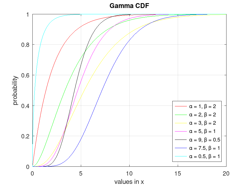
Example: 1
Plot various CDFs from the Gamma distribution
 x = 0:0.01:20;
 p1 = gamcdf (x, 1, 2);
 p2 = gamcdf (x, 2, 2);
 p3 = gamcdf (x, 3, 2);
 p4 = gamcdf (x, 5, 1);
 p5 = gamcdf (x, 9, 0.5);
 p6 = gamcdf (x, 7.5, 1);
 p7 = gamcdf (x, 0.5, 1);
 plot (x, p1, '-r', x, p2, '-g', x, p3, '-y', x, p4, '-m', ...
       x, p5, '-k', x, p6, '-b', x, p7, '-c')
 grid on
 legend ({'α = 1, β = 2', 'α = 2, β = 2', 'α = 3, β = 2', ...
          'α = 5, β = 1', 'α = 9, β = 0.5', 'α = 7.5, β = 1', ...
          'α = 0.5, β = 1'}, 'location', 'southeast')
 title ('Gamma CDF')
 xlabel ('values in x')
 ylabel ('probability')