Statistics: anovan

Function Reference: `anovan`

statistics: p = anovan (Y, GROUP)
statistics: p = anovan (Y, GROUP, name, value)
statistics: [p, atab] = anovan (…)
statistics: [p, atab, stats] = anovan (…)
statistics: [p, atab, stats, terms] = anovan (…)

Perform a multi (N)-way analysis of (co)variance (ANOVA or ANCOVA) to evaluate the effect of one or more categorical or continuous predictors (i.e. independent variables) on a continuous outcome (i.e. dependent variable). The algorithms used make anovan suitable for balanced or unbalanced factorial (crossed) designs. By default, anovan treats all factors as fixed. Examples of function usage can be found by entering the command demo anovan. A bootstrap resampling variant of this function, bootlm, is available in the statistics-resampling package and has similar usage.

Data is a single vector Y with groups specified by a corresponding matrix or cell array of group labels GROUP, where each column of GROUP has the same number of rows as Y. For example, if Y = [1.1;1.2]; GROUP = [1,2,1; 1,5,2]; then observation 1.1 was measured under conditions 1,2,1 and observation 1.2 was measured under conditions 1,5,2. If the GROUP provided is empty, then the linear model is fit with just the intercept (no predictors).

anovan can take a number of optional parameters as name-value pairs.

[…] = anovan (Y, GROUP, "continuous", continuous)

continuous is a vector of indices indicating which of the columns (i.e. factors) in GROUP should be treated as continuous predictors rather than as categorical predictors. The relationship between continuous predictors and the outcome should be linear.

[…] = anovan (Y, GROUP, "random", random)

random is a vector of indices indicating which of the columns (i.e. factors) in GROUP should be treated as random effects rather than fixed effects. Octave anovan provides only basic support for random effects. Specifically, since all F-statistics in anovan are calculated using the mean-squared error (MSE), any interaction terms containing a random effect are dropped from the model term definitions and their associated variance is pooled with the residual, unexplained variance making up the MSE. In effect, the model then fitted equates to a linear mixed model with random intercept(s). Variable names for random factors are appended with a ’ symbol.

[…] = anovan (Y, GROUP, "model", modeltype)

modeltype can specified as one of the following:
- "linear" (default) : compute $N$ main effects with no interactions.
- "interaction" : compute $N$ effects and $N×(N-1)$ two-factor interactions
- "full" : compute the $N$ main effects and interactions at all levels
- a scalar integer : representing the maximum interaction order
- a matrix of term definitions : each row is a term and each column is a factor
-- Example: A two-way ANOVA with interaction would be: [1 0; 0 1; 1 1]

[…] = anovan (Y, GROUP, "sstype", sstype)

sstype can specified as one of the following:
- 1 : Type I sequential sums-of-squares.
- 2 or "h" : Type II partially sequential (or hierarchical) sums-of-squares
- 3 (default) : Type III partial, constrained or marginal sums-of-squares

[…] = anovan (Y, GROUP, "varnames", varnames)

varnames must be a cell array of strings with each element containing a factor name for each column of GROUP. By default (if not parsed as optional argument), varnames are "X1","X2","X3", etc.

[…] = anovan (Y, GROUP, "alpha", alpha)

alpha must be a scalar value between 0 and 1 requesting $100×(1-$ alpha)% confidence bounds for the regression coefficients returned in stats.coeffs (default 0.05 for 95% confidence).

[…] = anovan (Y, GROUP, "display", dispopt)

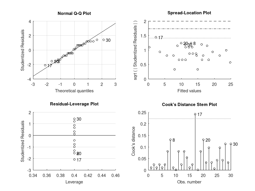
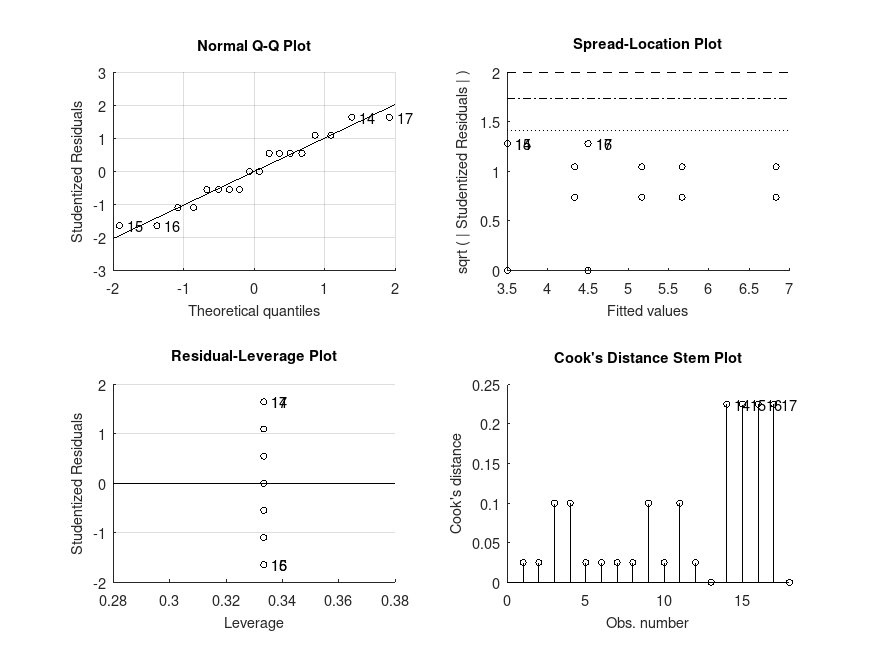
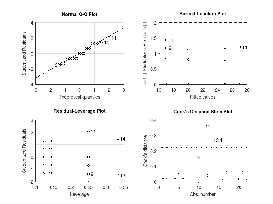
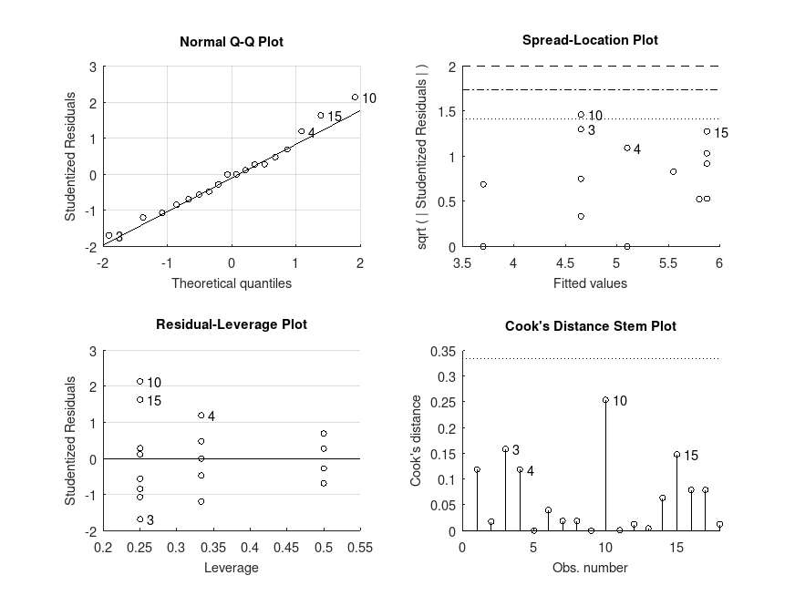
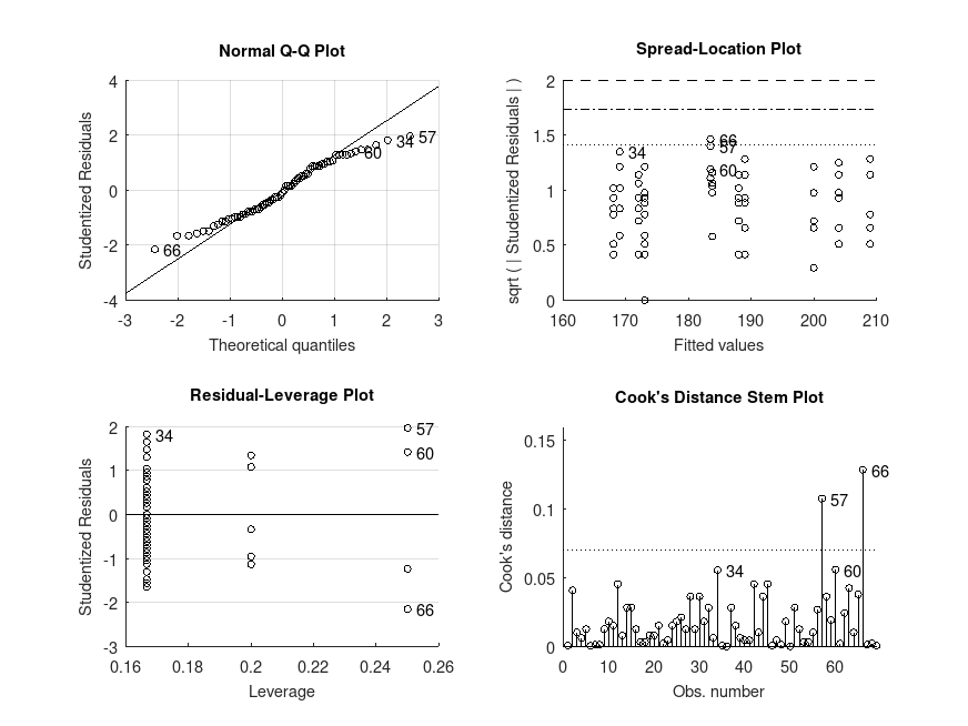
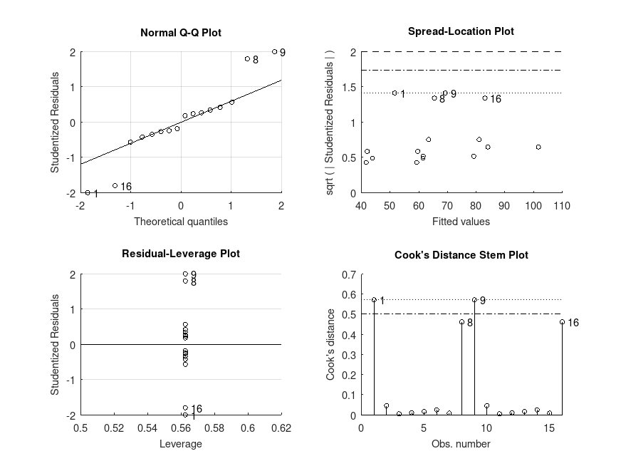
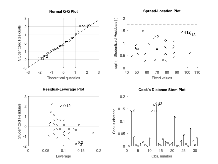
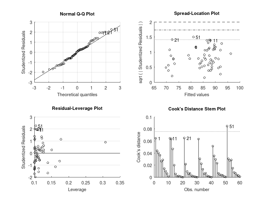
dispopt can be either "on" (default) or "off" and controls the display of the model formula, table of model parameters, the ANOVA table and the diagnostic plots. The F-statistic and p-values are formatted in APA-style. To avoid p-hacking, the table of model parameters is only displayed if we set planned contrasts (see below).

[…] = anovan (Y, GROUP, "contrasts", contrasts)

contrasts can be specified as one of the following:
- A string corresponding to one of the built-in contrasts listed below:
  - "simple" or "anova" (default): Simple (ANOVA) contrast coding. (The first level appearing in the GROUP column is the reference level)
  - "poly": Polynomial contrast coding for trend analysis.
  - "helmert": Helmert contrast coding: the difference between each level with the mean of the subsequent levels.
  - "effect": Deviation effect coding. (The first level appearing in the GROUP column is omitted).
  - "sdif" or "sdiff": Successive differences contrast coding: the difference between each level with the previous level.
  - "treatment": Treatment contrast (or dummy) coding. (The first level appearing in the GROUP column is the reference level). These contrasts are not compatible with sstype = 3.
- A matrix containing a custom contrast coding scheme (i.e. the generalized inverse of contrast weights). Rows in the contrast matrices correspond to factor levels in the order that they first appear in the GROUP column. The matrix must contain the same number of columns as there are the number of factor levels minus one.
If the anovan model contains more than one factor and a built-in contrast coding scheme was specified, then those contrasts are applied to all factors. To specify different contrasts for different factors in the model, contrasts should be a cell array with the same number of cells as there are columns in GROUP. Each cell should define contrasts for the respective column in GROUP by one of the methods described above. If cells are left empty, then the default contrasts are applied. Contrasts for cells corresponding to continuous factors are ignored.

[…] = anovan (Y, GROUP, "weights", weights)

weights is an optional vector of weights to be used when fitting the linear model. Weighted least squares (WLS) is used with weights (that is, minimizing sum (weights * residuals .^ 2)); otherwise ordinary least squares (OLS) is used (default is empty for OLS).

anovan can return up to four output arguments:

p = anovan (…) returns a vector of p-values, one for each term.

[p, atab] = anovan (…) returns a cell array containing the ANOVA table.

[p, atab, stats] = anovan (…) returns a structure containing additional statistics, including degrees of freedom and effect sizes for each term in the linear model, the design matrix, the variance-covariance matrix, (weighted) model residuals, and the mean squared error. The columns of stats.coeffs (from left-to-right) report the model coefficients, standard errors, lower and upper $100×(1-alpha)%$ confidence interval bounds, t-statistics, and p-values relating to the contrasts. The number appended to each term name in stats.coeffnames corresponds to the column number in the relevant contrast matrix for that factor. The stats structure can be used as input for multcompare.

[p, atab, stats, terms] = anovan (…) returns the model term definitions.

See also: anova1, anova2, multcompare, fitlm

Source Code: anovan

Example: 1



 # Two-sample unpaired test on independent samples (equivalent to Student's
 # t-test). Note that the absolute value of t-statistic can be obtained by
 # taking the square root of the reported F statistic. In this example,
 # t = sqrt (1.44) = 1.20.

 score = [54 23 45 54 45 43 34 65 77 46 65]';
 gender = {"male" "male" "male" "male" "male" "female" "female" "female" ...
           "female" "female" "female"}';

 [P, ATAB, STATS] = anovan (score, gender, "display", "on", "varnames", "gender");


MODEL FORMULA (based on Wilkinson's notation):

Y ~ 1 + gender

ANOVA TABLE (Type III sums-of-squares):

Source                   Sum Sq.    d.f.    Mean Sq.  R Sq.            F  Prob>F
--------------------------------------------------------------------------------
gender                    318.11       1      318.11  0.138         1.44    .261 
Error                     1992.8       9      221.42
Total                     2310.9      10

Example: 2



 # Two-sample paired test on dependent or matched samples equivalent to a
 # paired t-test. As for the first example, the t-statistic can be obtained by
 # taking the square root of the reported F statistic. Note that the interaction
 # between treatment x subject was dropped from the full model by assigning
 # subject as a random factor (').

 score = [4.5 5.6; 3.7 6.4; 5.3 6.4; 5.4 6.0; 3.9 5.7]';
 treatment = {"before" "after"; "before" "after"; "before" "after";
              "before" "after"; "before" "after"}';
 subject = {"GS" "GS"; "JM" "JM"; "HM" "HM"; "JW" "JW"; "PS" "PS"}';

 [P, ATAB, STATS] = anovan (score(:), {treatment(:), subject(:)}, ...
                            "model", "full", "random", 2, "sstype", 2, ...
                            "varnames", {"treatment", "subject"}, ...
                            "display", "on");


MODEL FORMULA (based on Wilkinson's notation):

Y ~ 1 + treatment + (1|subject)

ANOVA TABLE (Type II sums-of-squares):

Source                   Sum Sq.    d.f.    Mean Sq.  R Sq.            F  Prob>F
--------------------------------------------------------------------------------
treatment                  5.329       1       5.329  0.801        16.08    .016 
subject'                   1.674       4      0.4185  0.558         1.26    .413 
Error                      1.326       4      0.3315
Total                      8.329       9

Example: 3



 # One-way ANOVA on the data from a study on the strength of structural beams,
 # in Hogg and Ledolter (1987) Engineering Statistics. New York: MacMillan

 strength = [82 86 79 83 84 85 86 87 74 82 ...
            78 75 76 77 79 79 77 78 82 79]';
 alloy = {"st","st","st","st","st","st","st","st", ...
          "al1","al1","al1","al1","al1","al1", ...
          "al2","al2","al2","al2","al2","al2"}';

 [P, ATAB, STATS] = anovan (strength, alloy, "display", "on", ...
                            "varnames", "alloy");


MODEL FORMULA (based on Wilkinson's notation):

Y ~ 1 + alloy

ANOVA TABLE (Type III sums-of-squares):

Source                   Sum Sq.    d.f.    Mean Sq.  R Sq.            F  Prob>F
--------------------------------------------------------------------------------
alloy                      184.8       2        92.4  0.644        15.40   <.001 
Error                        102      17           6
Total                      286.8      19

Example: 4



 # One-way repeated measures ANOVA on the data from a study on the number of
 # words recalled by 10 subjects for three time condtions, in Loftus & Masson
 # (1994) Psychon Bull Rev. 1(4):476-490, Table 2. Note that the interaction
 # between seconds x subject was dropped from the full model by assigning
 # subject as a random factor (').

 words = [10 13 13; 6 8 8; 11 14 14; 22 23 25; 16 18 20; ...
          15 17 17; 1 1 4; 12 15 17;  9 12 12;  8 9 12];
 seconds = [1 2 5; 1 2 5; 1 2 5; 1 2 5; 1 2 5; ...
            1 2 5; 1 2 5; 1 2 5; 1 2 5; 1 2 5;];
 subject = [ 1  1  1;  2  2  2;  3  3  3;  4  4  4;  5  5  5; ...
             6  6  6;  7  7  7;  8  8  8;  9  9  9; 10 10 10];

 [P, ATAB, STATS] = anovan (words(:), {seconds(:), subject(:)}, ...
                            "model", "full", "random", 2, "sstype", 2, ...
                            "display", "on", "varnames", {"seconds", "subject"});


MODEL FORMULA (based on Wilkinson's notation):

Y ~ 1 + seconds + (1|subject)

ANOVA TABLE (Type II sums-of-squares):

Source                   Sum Sq.    d.f.    Mean Sq.  R Sq.            F  Prob>F
--------------------------------------------------------------------------------
seconds                   52.267       2      26.133  0.825        42.51   <.001 
subject'                  942.53       9      104.73  0.988       170.34   <.001 
Error                     11.067      18     0.61481
Total                     1005.9      29

Example: 5



 # Balanced two-way ANOVA with interaction on the data from a study of popcorn
 # brands and popper types, in Hogg and Ledolter (1987) Engineering Statistics.
 # New York: MacMillan

 popcorn = [5.5, 4.5, 3.5; 5.5, 4.5, 4.0; 6.0, 4.0, 3.0; ...
            6.5, 5.0, 4.0; 7.0, 5.5, 5.0; 7.0, 5.0, 4.5];
 brands = {"Gourmet", "National", "Generic"; ...
           "Gourmet", "National", "Generic"; ...
           "Gourmet", "National", "Generic"; ...
           "Gourmet", "National", "Generic"; ...
           "Gourmet", "National", "Generic"; ...
           "Gourmet", "National", "Generic"};
 popper = {"oil", "oil", "oil"; "oil", "oil", "oil"; "oil", "oil", "oil"; ...
           "air", "air", "air"; "air", "air", "air"; "air", "air", "air"};

 [P, ATAB, STATS] = anovan (popcorn(:), {brands(:), popper(:)}, ...
                            "display", "on", "model", "full", ...
                            "varnames", {"brands", "popper"});


MODEL FORMULA (based on Wilkinson's notation):

Y ~ 1 + brands + popper + brands:popper

ANOVA TABLE (Type III sums-of-squares):

Source                   Sum Sq.    d.f.    Mean Sq.  R Sq.            F  Prob>F
--------------------------------------------------------------------------------
brands                     15.75       2       7.875  0.904        56.70   <.001 
popper                       4.5       1         4.5  0.730        32.40   <.001 
brands*popper           0.083333       2    0.041667  0.048         0.30    .746 
Error                     1.6667      12     0.13889
Total                         22      17

Example: 6



 # Unbalanced two-way ANOVA (2x2) on the data from a study on the effects of
 # gender and having a college degree on salaries of company employees,
 # in Maxwell, Delaney and Kelly (2018): Chapter 7, Table 15

 salary = [24 26 25 24 27 24 27 23 15 17 20 16, ...
           25 29 27 19 18 21 20 21 22 19]';
 gender = {"f" "f" "f" "f" "f" "f" "f" "f" "f" "f" "f" "f"...
           "m" "m" "m" "m" "m" "m" "m" "m" "m" "m"}';
 degree = [1 1 1 1 1 1 1 1 0 0 0 0 1 1 1 0 0 0 0 0 0 0]';

 [P, ATAB, STATS] = anovan (salary, {gender, degree}, "model", "full", ...
                            "sstype", 3, "display", "on", "varnames", ...
                            {"gender", "degree"});


MODEL FORMULA (based on Wilkinson's notation):

Y ~ 1 + gender + degree + gender:degree

ANOVA TABLE (Type III sums-of-squares):

Source                   Sum Sq.    d.f.    Mean Sq.  R Sq.            F  Prob>F
--------------------------------------------------------------------------------
gender                    29.371       1      29.371  0.370        10.57    .004 
degree                    264.34       1      264.34  0.841        95.16   <.001 
gender*degree             1.1748       1      1.1748  0.023         0.42    .524 
Error                         50      18      2.7778
Total                     323.86      21

Example: 7



 # Unbalanced two-way ANOVA (3x2) on the data from a study of the effect of
 # adding sugar and/or milk on the tendency of coffee to make people babble,
 # in from Navarro (2019): 16.10

 sugar = {"real" "fake" "fake" "real" "real" "real" "none" "none" "none" ...
          "fake" "fake" "fake" "real" "real" "real" "none" "none" "fake"}';
 milk = {"yes" "no" "no" "yes" "yes" "no" "yes" "yes" "yes" ...
         "no" "no" "yes" "no" "no" "no" "no" "no" "yes"}';
 babble = [4.6 4.4 3.9 5.6 5.1 5.5 3.9 3.5 3.7...
           5.6 4.7 5.9 6.0 5.4 6.6 5.8 5.3 5.7]';

 [P, ATAB, STATS] = anovan (babble, {sugar, milk}, "model", "full",  ...
                            "sstype", 3, "display", "on", ...
                            "varnames", {"sugar", "milk"});


MODEL FORMULA (based on Wilkinson's notation):

Y ~ 1 + sugar + milk + sugar:milk

ANOVA TABLE (Type III sums-of-squares):

Source                   Sum Sq.    d.f.    Mean Sq.  R Sq.            F  Prob>F
--------------------------------------------------------------------------------
sugar                     2.1318       2      1.0659  0.403         4.04    .045 
milk                      1.0041       1      1.0041  0.241         3.81    .075 
sugar*milk                5.9439       2      2.9719  0.653        11.28    .002 
Error                     3.1625      12     0.26354
Total                      13.62      17

Example: 8



 # Unbalanced three-way ANOVA (3x2x2) on the data from a study of the effects
 # of three different drugs, biofeedback and diet on patient blood pressure,
 # adapted* from Maxwell, Delaney and Kelly (2018): Chapter 8, Table 12
 # * Missing values introduced to make the sample sizes unequal to test the
 #   calculation of different types of sums-of-squares

 drug = {"X" "X" "X" "X" "X" "X" "X" "X" "X" "X" "X" "X" ...
         "X" "X" "X" "X" "X" "X" "X" "X" "X" "X" "X" "X";
         "Y" "Y" "Y" "Y" "Y" "Y" "Y" "Y" "Y" "Y" "Y" "Y" ...
         "Y" "Y" "Y" "Y" "Y" "Y" "Y" "Y" "Y" "Y" "Y" "Y";
         "Z" "Z" "Z" "Z" "Z" "Z" "Z" "Z" "Z" "Z" "Z" "Z" ...
         "Z" "Z" "Z" "Z" "Z" "Z" "Z" "Z" "Z" "Z" "Z" "Z"};
 feedback = [1 1 1 1 1 1 1 1 1 1 1 1 0 0 0 0 0 0 0 0 0 0 0 0;
             1 1 1 1 1 1 1 1 1 1 1 1 0 0 0 0 0 0 0 0 0 0 0 0;
             1 1 1 1 1 1 1 1 1 1 1 1 0 0 0 0 0 0 0 0 0 0 0 0];
 diet = [0 0 0 0 0 0 1 1 1 1 1 1 0 0 0 0 0 0 1 1 1 1 1 1;
         0 0 0 0 0 0 1 1 1 1 1 1 0 0 0 0 0 0 1 1 1 1 1 1;
         0 0 0 0 0 0 1 1 1 1 1 1 0 0 0 0 0 0 1 1 1 1 1 1];
 BP = [170 175 165 180 160 158 161 173 157 152 181 190 ...
       173 194 197 190 176 198 164 190 169 164 176 175;
       186 194 201 215 219 209 164 166 159 182 187 174 ...
       189 194 217 206 199 195 171 173 196 199 180 NaN;
       180 187 199 170 204 194 162 184 183 156 180 173 ...
       202 228 190 206 224 204 205 199 170 160 NaN NaN];

 [P, ATAB, STATS] = anovan (BP(:), {drug(:), feedback(:), diet(:)}, ...
                                    "model", "full", "sstype", 3, ...
                                    "display", "on", ...
                                    "varnames", {"drug", "feedback", "diet"});


MODEL FORMULA (based on Wilkinson's notation):

Y ~ 1 + drug + feedback + diet + drug:feedback + drug:diet + feedback:diet + drug:feedback:diet

ANOVA TABLE (Type III sums-of-squares):

Source                   Sum Sq.    d.f.    Mean Sq.  R Sq.            F  Prob>F
--------------------------------------------------------------------------------
drug                      3430.9       2      1715.4  0.275        10.79   <.001 
feedback                  1833.7       1      1833.7  0.168        11.53    .001 
diet                      5080.5       1      5080.5  0.359        31.94   <.001 
drug*feedback             382.08       2      191.04  0.040         1.20    .308 
drug*diet                 963.04       2      481.52  0.096         3.03    .056 
feedback*diet             44.452       1      44.452  0.005         0.28    .599 
drug*feedback*diet        814.35       2      407.17  0.082         2.56    .086 
Error                     9065.8      57      159.05
Total                      22190      68

Example: 9



 # Balanced three-way ANOVA (2x2x2) with one of the factors being a blocking
 # factor. The data is from a randomized block design study on the effects
 # of antioxidant treatment on glutathione-S-transferase (GST) levels in
 # different mouse strains, from Festing (2014), ILAR Journal, 55(3):427-476.
 # Note that all interactions involving block were dropped from the full model
 # by assigning block as a random factor (').

 measurement = [444 614 423 625 408  856 447 719 ...
                764 831 586 782 609 1002 606 766]';
 strain= {"NIH","NIH","BALB/C","BALB/C","A/J","A/J","129/Ola","129/Ola", ...
          "NIH","NIH","BALB/C","BALB/C","A/J","A/J","129/Ola","129/Ola"}';
 treatment={"C" "T" "C" "T" "C" "T" "C" "T" "C" "T" "C" "T" "C" "T" "C" "T"}';
 block = [1 1 1 1 1 1 1 1 2 2 2 2 2 2 2 2]';

 [P, ATAB, STATS] = anovan (measurement/10, {strain, treatment, block}, ...
                            "sstype", 2, "model", "full", "random", 3, ...
                            "display", "on", ...
                            "varnames", {"strain", "treatment", "block"});


MODEL FORMULA (based on Wilkinson's notation):

Y ~ 1 + strain + treatment + (1|block) + strain:treatment

ANOVA TABLE (Type II sums-of-squares):

Source                   Sum Sq.    d.f.    Mean Sq.  R Sq.            F  Prob>F
--------------------------------------------------------------------------------
strain                    286.13       3      95.378  0.580         3.23    .091 
treatment                 2275.3       1      2275.3  0.917        76.94   <.001 
block'                    1242.6       1      1242.6  0.857        42.02   <.001 
strain*treatment           495.9       3       165.3  0.706         5.59    .028 
Error                     207.01       7      29.573
Total                     4506.9      15

Example: 10



 # One-way ANCOVA on data from a study of the additive effects of species
 # and temperature on chirpy pulses of crickets, from Stitch, The Worst Stats
 # Text eveR

 pulse = [67.9 65.1 77.3 78.7 79.4 80.4 85.8 86.6 87.5 89.1 ...
          98.6 100.8 99.3 101.7 44.3 47.2 47.6 49.6 50.3 51.8 ...
          60 58.5 58.9 60.7 69.8 70.9 76.2 76.1 77 77.7 84.7]';
 temp = [20.8 20.8 24 24 24 24 26.2 26.2 26.2 26.2 28.4 ...
         29 30.4 30.4 17.2 18.3 18.3 18.3 18.9 18.9 20.4 ...
         21 21 22.1 23.5 24.2 25.9 26.5 26.5 26.5 28.6]';
 species = {"ex" "ex" "ex" "ex" "ex" "ex" "ex" "ex" "ex" "ex" "ex" ...
            "ex" "ex" "ex" "niv" "niv" "niv" "niv" "niv" "niv" "niv" ...
            "niv" "niv" "niv" "niv" "niv" "niv" "niv" "niv" "niv" "niv"};

 [P, ATAB, STATS] = anovan (pulse, {species, temp}, "model", "linear", ...
                           "continuous", 2, "sstype", "h", "display", "on", ...
                           "varnames", {"species", "temp"});


MODEL FORMULA (based on Wilkinson's notation):

Y ~ 1 + species + temp

ANOVA TABLE (Type II sums-of-squares):

Source                   Sum Sq.    d.f.    Mean Sq.  R Sq.            F  Prob>F
--------------------------------------------------------------------------------
species                      598       1         598  0.870       187.40   <.001 
temp                      4376.1       1      4376.1  0.980      1371.35   <.001 
Error                      89.35      28      3.1911
Total                     8582.2      30

Example: 11



 # Factorial ANCOVA on data from a study of the effects of treatment and
 # exercise on stress reduction score after adjusting for age. Data from R
 # datarium package).

 score = [95.6 82.2 97.2 96.4 81.4 83.6 89.4 83.8 83.3 85.7 ...
          97.2 78.2 78.9 91.8 86.9 84.1 88.6 89.8 87.3 85.4 ...
          81.8 65.8 68.1 70.0 69.9 75.1 72.3 70.9 71.5 72.5 ...
          84.9 96.1 94.6 82.5 90.7 87.0 86.8 93.3 87.6 92.4 ...
          100. 80.5 92.9 84.0 88.4 91.1 85.7 91.3 92.3 87.9 ...
          91.7 88.6 75.8 75.7 75.3 82.4 80.1 86.0 81.8 82.5]';
 treatment = {"yes" "yes" "yes" "yes" "yes" "yes" "yes" "yes" "yes" "yes" ...
              "yes" "yes" "yes" "yes" "yes" "yes" "yes" "yes" "yes" "yes" ...
              "yes" "yes" "yes" "yes" "yes" "yes" "yes" "yes" "yes" "yes" ...
              "no"  "no"  "no"  "no"  "no"  "no"  "no"  "no"  "no"  "no"  ...
              "no"  "no"  "no"  "no"  "no"  "no"  "no"  "no"  "no"  "no"  ...
              "no"  "no"  "no"  "no"  "no"  "no"  "no"  "no"  "no"  "no"}';
 exercise = {"lo"  "lo"  "lo"  "lo"  "lo"  "lo"  "lo"  "lo"  "lo"  "lo"  ...
             "mid" "mid" "mid" "mid" "mid" "mid" "mid" "mid" "mid" "mid" ...
             "hi"  "hi"  "hi"  "hi"  "hi"  "hi"  "hi"  "hi"  "hi"  "hi"  ...
             "lo"  "lo"  "lo"  "lo"  "lo"  "lo"  "lo"  "lo"  "lo"  "lo"  ...
             "mid" "mid" "mid" "mid" "mid" "mid" "mid" "mid" "mid" "mid" ...
             "hi"  "hi"  "hi"  "hi"  "hi"  "hi"  "hi"  "hi"  "hi"  "hi"}';
 age = [59 65 70 66 61 65 57 61 58 55 62 61 60 59 55 57 60 63 62 57 ...
        58 56 57 59 59 60 55 53 55 58 68 62 61 54 59 63 60 67 60 67 ...
        75 54 57 62 65 60 58 61 65 57 56 58 58 58 52 53 60 62 61 61]';

 [P, ATAB, STATS] = anovan (score, {treatment, exercise, age}, ...
                            "model", [1 0 0; 0 1 0; 0 0 1; 1 1 0], ...
                            "continuous", 3, "sstype", "h", "display", "on", ...
                            "varnames", {"treatment", "exercise", "age"});


MODEL FORMULA (based on Wilkinson's notation):

Y ~ 1 + treatment + exercise + age + treatment:exercise

ANOVA TABLE (Type II sums-of-squares):

Source                   Sum Sq.    d.f.    Mean Sq.  R Sq.            F  Prob>F
--------------------------------------------------------------------------------
treatment                  275.7       1       275.7  0.173        11.10    .002 
exercise                  1034.6       2      517.32  0.440        20.82   <.001 
age                       226.36       1      226.36  0.147         9.11    .004 
treatment*exercise        220.94       2      110.47  0.144         4.45    .016 
Error                     1316.9      53      24.848
Total                     3888.3      59

Example: 12



 # Unbalanced one-way ANOVA with custom, orthogonal contrasts. The statistics
 # relating to the contrasts are shown in the table of model parameters, and
 # can be retrieved from the STATS.coeffs output.

 dv =  [ 8.706 10.362 11.552  6.941 10.983 10.092  6.421 14.943 15.931 ...
        22.968 18.590 16.567 15.944 21.637 14.492 17.965 18.851 22.891 ...
        22.028 16.884 17.252 18.325 25.435 19.141 21.238 22.196 18.038 ...
        22.628 31.163 26.053 24.419 32.145 28.966 30.207 29.142 33.212 ...
        25.694 ]';
 g = [1 1 1 1 1 1 1 1 2 2 2 2 2 3 3 3 3 3 3 3 3 ...
      4 4 4 4 4 4 4 5 5 5 5 5 5 5 5 5]';
 C = [ 0.4001601  0.3333333  0.5  0.0
       0.4001601  0.3333333 -0.5  0.0
       0.4001601 -0.6666667  0.0  0.0
      -0.6002401  0.0000000  0.0  0.5
      -0.6002401  0.0000000  0.0 -0.5];

 [P,ATAB, STATS] = anovan (dv, g, "contrasts", C, "varnames", "score", ...
                          "alpha", 0.05, "display", "on");


MODEL FORMULA (based on Wilkinson's notation):

Y ~ 1 + score

MODEL PARAMETERS (contrasts for the fixed effects)

Parameter               Estimate        SE  Lower.CI  Upper.CI        t Prob>|t|
--------------------------------------------------------------------------------
(Intercept)                 19.4     0.483      18.4      20.4    40.16    <.001 
score_1                    -9.33     0.969     -11.3     -7.36    -9.62    <.001 
score_2                       -5      1.31     -7.66     -2.34    -3.82    <.001 
score_3                       -8      1.64     -11.3     -4.66    -4.87    <.001 
score_4                       -8      1.45       -11     -5.04    -5.51    <.001 

ANOVA TABLE (Type III sums-of-squares):

Source                   Sum Sq.    d.f.    Mean Sq.  R Sq.            F  Prob>F
--------------------------------------------------------------------------------
score                     1561.3       4      390.33  0.855        47.10   <.001 
Error                     265.17      32      8.2866
Total                     1826.5      36

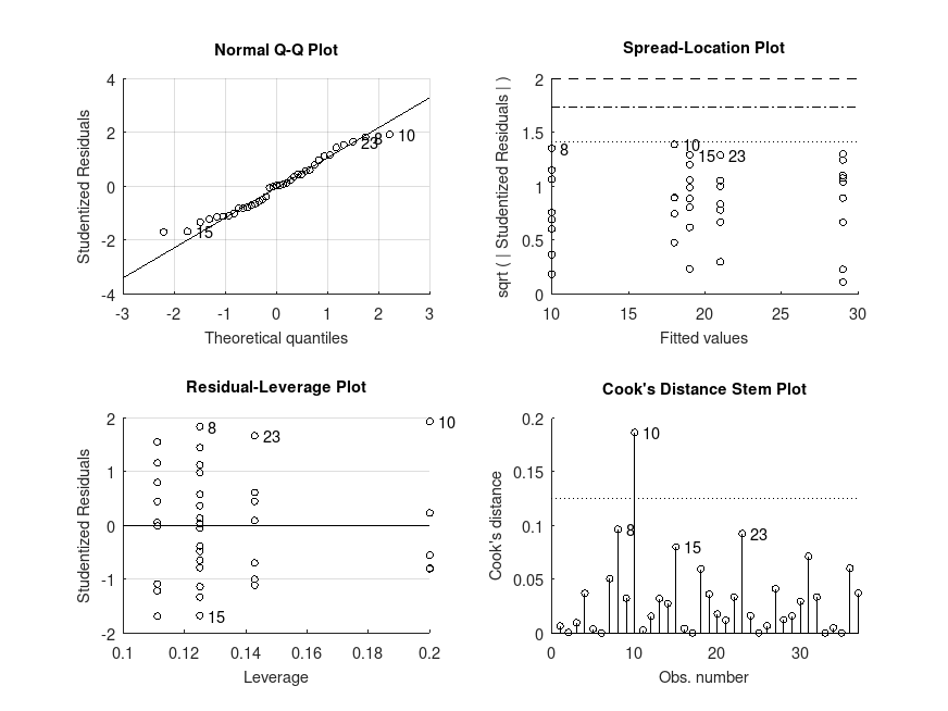
Example: 13



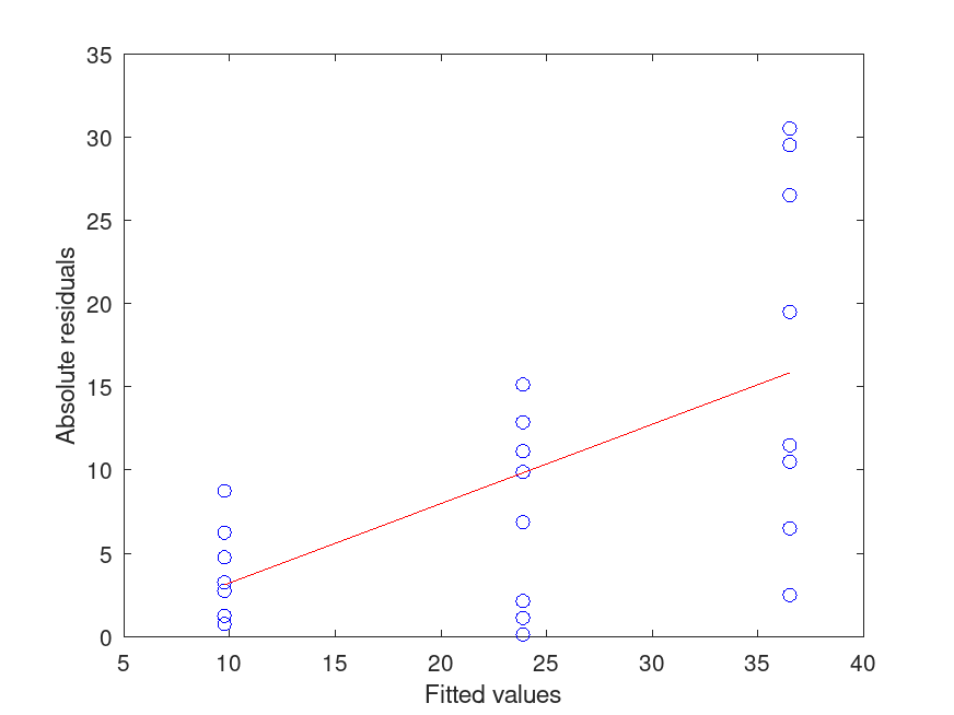
 # One-way ANOVA with the linear model fit by weighted least squares to
 # account for heteroskedasticity. In this example, the variance appears
 # proportional to the outcome, so weights have been estimated by initially
 # fitting the model without weights and regressing the absolute residuals on
 # the fitted values. Although this data could have been analysed by Welch's
 # ANOVA test, the approach here can generalize to ANOVA models with more than
 # one factor.

 g = [1, 1, 1, 1, 1, 1, 1, 1, ...
      2, 2, 2, 2, 2, 2, 2, 2, ...
      3, 3, 3, 3, 3, 3, 3, 3]';
 y = [13, 16, 16,  7, 11,  5,  1,  9, ...
      10, 25, 66, 43, 47, 56,  6, 39, ...
      11, 39, 26, 35, 25, 14, 24, 17]';

 [P,ATAB,STATS] = anovan(y, g, "display", "off");
 fitted = STATS.X * STATS.coeffs(:,1); # fitted values
 b = polyfit (fitted, abs (STATS.resid), 1);
 v = polyval (b, fitted);  # Variance as a function of the fitted values
 figure("Name", "Regression of the absolute residuals on the fitted values");
 plot (fitted, abs (STATS.resid),'ob');hold on; plot(fitted,v,'-r'); hold off;
 xlabel("Fitted values"); ylabel("Absolute residuals");

 [P,ATAB,STATS] = anovan (y, g, "weights", v.^-1);


MODEL FORMULA (based on Wilkinson's notation):

Y ~ 1 + X1

ANOVA TABLE (Type III sums-of-squares):

Source                   Sum Sq.    d.f.    Mean Sq.  R Sq.            F  Prob>F
--------------------------------------------------------------------------------
X1                        2237.9       2      1118.9  0.522        11.49   <.001 
Error                     2045.5      21      97.405
Total                     6905.6      23

Function Reference: anovan