Categories &
Functions List
- adtest
- anova
- anova1
- anova2
- anovan
- ansaribradley
- barttest
- binotest
- chi2gof
- chi2test
- correlation_test
- detectdrift
- dwtest
- fishertest
- friedman
- hotelling_t2test
- hotelling_t2test2
- jbtest
- knntest
- kruskalwallis
- kstest
- kstest2
- lillietest
- manova1
- mcnemar_test
- meanEffectSize
- mmdtest
- multcompare
- ranksum
- regression_ftest
- regression_ttest
- runstest
- signrank
- signtest
- stats.drift.DriftDiagnostics
- swtest
- ttest
- ttest2
- vartest
- vartest2
- vartestn
- ztest
- ztest2
- CompactLinearModel
- CoxModel
- coxphfit
- fitcox
- fitglm
- fitglme
- fitlm
- fitlme
- fitlmematrix
- fitnlm
- fitrm
- GeneralizedLinearMixedModel
- GeneralizedLinearModel
- glmfit
- glmval
- invpred
- lasso
- lassoglm
- LinearFormula
- LinearMixedModel
- LinearModel
- logistic_regression
- mnrfit
- mnrval
- monotone_smooth
- mvregress
- mvregresslike
- nlinfit
- nlparci
- nlpredci
- NonLinearModel
- plsregress
- regress
- regress_gp
- RepeatedMeasuresModel
- ridge
- robustfit
- stepwisefit
- stepwiseglm
- stepwiselm
- ClassificationBaggedEnsemble
- ClassificationDiscriminant
- ClassificationECOC
- ClassificationEnsemble
- ClassificationGAM
- ClassificationKernel
- ClassificationKNN
- ClassificationLinear
- ClassificationNaiveBayes
- ClassificationNeuralNetwork
- ClassificationPartitionedECOC
- ClassificationPartitionedEnsemble
- ClassificationPartitionedKernel
- ClassificationPartitionedLinear
- ClassificationPartitionedModel
- ClassificationSVM
- ClassificationTree
- CompactClassificationDiscriminant
- CompactClassificationECOC
- CompactClassificationEnsemble
- CompactClassificationGAM
- CompactClassificationNaiveBayes
- CompactClassificationNeuralNetwork
- CompactClassificationSVM
- CompactClassificationTree
- CompactRegressionGAM
- CompactRegressionEnsemble
- CompactRegressionGP
- CompactRegressionNeuralNetwork
- CompactRegressionSVM
- CompactRegressionTree
- CompactTreeBagger
- designecoc
- fcnnpredict
- fcnntrain
- fitcdiscr
- fitcecoc
- fitcensemble
- fitcgam
- fitckernel
- fitcknn
- fitclinear
- fitcnb
- fitcnet
- fitcsvm
- fitctree
- fitrensemble
- fitrgam
- fitrgp
- fitrkernel
- fitrlinear
- fitrnet
- fitrsvm
- fitrtree
- gamboostinter
- gamboostpairs
- gamboostpredict
- gamboosttrain
- gampredict
- gamtrain
- partialDependence
- plotPartialDependence
- PredictiveModel
- RegressionBaggedEnsemble
- RegressionEnsemble
- RegressionGAM
- RegressionGP
- RegressionKernel
- RegressionLinear
- RegressionNeuralNetwork
- RegressionPartitionedEnsemble
- RegressionPartitionedKernel
- RegressionPartitionedLinear
- RegressionPartitionedModel
- RegressionSVM
- RegressionTree
- lime
- shapley
- svmpredict
- svmtrain
- templateDiscriminant
- templateEnsemble
- templateKernel
- templateKNN
- templateLinear
- templateNaiveBayes
- templateSVM
- templateTree
- TreeBagger
- treepredict
- treetrain
- paretotails
- prob.ProbabilityDistribution
- prob.BetaDistribution
- prob.BinomialDistribution
- prob.BirnbaumSaundersDistribution
- prob.BurrDistribution
- prob.ExponentialDistribution
- prob.ExtremeValueDistribution
- prob.GammaDistribution
- prob.GeneralizedExtremeValueDistribution
- prob.GeneralizedParetoDistribution
- prob.HalfNormalDistribution
- prob.InverseGaussianDistribution
- prob.KernelDistribution
- prob.LogisticDistribution
- prob.LoglogisticDistribution
- prob.LognormalDistribution
- prob.LoguniformDistribution
- prob.MultinomialDistribution
- prob.NakagamiDistribution
- prob.NegativeBinomialDistribution
- prob.NormalDistribution
- prob.PiecewiseLinearDistribution
- prob.PoissonDistribution
- prob.RayleighDistribution
- prob.RicianDistribution
- prob.StableDistribution
- prob.tLocationScaleDistribution
- prob.TriangularDistribution
- prob.UniformDistribution
- prob.WeibullDistribution
- betafit
- betalike
- binofit
- binolike
- bisafit
- bisalike
- burrfit
- burrlike
- copulafit
- evfit
- evlike
- expfit
- explike
- gamfit
- gamlike
- geofit
- gevfit
- gevlike
- gevfit_lmom
- gpfit
- gplike
- gumbelfit
- gumbellike
- hnfit
- hnlike
- invgfit
- invglike
- logifit
- logilike
- loglfit
- logllike
- lognfit
- lognlike
- nakafit
- nakalike
- nbinfit
- nbinlike
- normfit
- normlike
- poissfit
- poisslike
- raylfit
- rayllike
- ricefit
- ricelike
- stblfit
- stbllike
- tlsfit
- tlslike
- unidfit
- unifit
- wblfit
- wbllike
- betacdf
- betainv
- betapdf
- betarnd
- binocdf
- binoinv
- binopdf
- binornd
- bisacdf
- bisainv
- bisapdf
- bisarnd
- burrcdf
- burrinv
- burrpdf
- burrrnd
- bvncdf
- bvtcdf
- cauchycdf
- cauchyinv
- cauchypdf
- cauchyrnd
- chi2cdf
- chi2inv
- chi2pdf
- chi2rnd
- copulacdf
- copulapdf
- copularnd
- evcdf
- evinv
- evpdf
- evrnd
- expcdf
- expinv
- exppdf
- exprnd
- fcdf
- finv
- fpdf
- frnd
- gamcdf
- gaminv
- gampdf
- gamrnd
- geocdf
- geoinv
- geopdf
- geornd
- gevcdf
- gevinv
- gevpdf
- gevrnd
- gpcdf
- gpinv
- gppdf
- gprnd
- gumbelcdf
- gumbelinv
- gumbelpdf
- gumbelrnd
- hncdf
- hninv
- hnpdf
- hnrnd
- hygecdf
- hygeinv
- hygepdf
- hygernd
- invgcdf
- invginv
- invgpdf
- invgrnd
- iwishpdf
- iwishrnd
- jsucdf
- jsupdf
- laplacecdf
- laplaceinv
- laplacepdf
- laplacernd
- logicdf
- logiinv
- logipdf
- logirnd
- loglcdf
- loglinv
- loglpdf
- loglrnd
- logncdf
- logninv
- lognpdf
- lognrnd
- mnpdf
- mnrnd
- mvncdf
- mvnpdf
- mvnrnd
- mvtcdf
- mvtpdf
- mvtrnd
- nakacdf
- nakainv
- nakapdf
- nakarnd
- nbincdf
- nbininv
- nbinpdf
- nbinrnd
- ncfcdf
- ncfinv
- ncfpdf
- ncfrnd
- nctcdf
- nctinv
- nctpdf
- nctrnd
- ncx2cdf
- ncx2inv
- ncx2pdf
- ncx2rnd
- normcdf
- norminv
- normpdf
- normrnd
- plcdf
- plinv
- plpdf
- plrnd
- poisscdf
- poissinv
- poisspdf
- poissrnd
- raylcdf
- raylinv
- raylpdf
- raylrnd
- ricecdf
- riceinv
- ricepdf
- ricernd
- stblcdf
- stblinv
- stblpdf
- stblrnd
- stdrcdf
- stdrinv
- stdrpdf
- stdrrnd
- tcdf
- tinv
- tpdf
- trnd
- tlscdf
- tlsinv
- tlspdf
- tlsrnd
- tricdf
- triinv
- tripdf
- trirnd
- unidcdf
- unidinv
- unidpdf
- unidrnd
- unifcdf
- unifinv
- unifpdf
- unifrnd
- vmcdf
- vminv
- vmpdf
- vmrnd
- wblcdf
- wblinv
- wblpdf
- wblrnd
- wienrnd
- wishpdf
- wishrnd
- betastat
- binostat
- bisastat
- burrstat
- chi2stat
- copulaparam
- copulastat
- evstat
- expstat
- fstat
- gamstat
- geostat
- gevstat
- gpstat
- gumbelstat
- hnstat
- hygestat
- invgstat
- logistat
- loglstat
- lognstat
- nakastat
- nbinstat
- ncfstat
- nctstat
- ncx2stat
- normstat
- plstat
- poisstat
- raylstat
- ricestat
- stdrstat
- tlsstat
- tristat
- tstat
- unidstat
- unifstat
- wblstat
- andrewsplot
- bar3
- bar3h
- biplot
- boxchart
- boxplot
- cdfplot
- dendrogram
- ecdfhist
- einstein
- gardnerAltmanPlot
- glyphplot
- gplotmatrix
- gscatter
- heatmap
- hist3
- histfit
- manovacluster
- normplot
- parallelcoords
- parallelplot
- ppplot
- probplot
- qqplot
- scatterhist
- scatterhistogram
- silhouette
- stats.chart.BoxChart
- stats.chart.HeatmapChart
- stats.chart.ParallelCoordinatesPlot
- stats.chart.ScatterHistogramChart
- swarmchart
- violin
- wblplot
Function Reference: fitcdiscr
statistics: Mdl = fitcdiscr (X, Y)
statistics: Mdl = fitcdiscr (Tbl, ResponseVarName)
statistics: Mdl = fitcdiscr (Tbl, formula)
statistics: Mdl = fitcdiscr (Tbl, Y)
statistics: Mdl = fitcdiscr (…, name, value)
Fit a Linear Discriminant Analysis classification model.
Mdl = fitcdiscr (X, Y) returns a Linear Discriminant
Analysis (LDA) classification model, Mdl, with X being the
predictor data, and Y the class labels of observations in X.
-
Xmust be a N×P numeric matrix of predictor data where rows correspond to observations and columns correspond to features or variables. -
Yis N×1 matrix or cell matrix containing the class labels of corresponding predictor data in X. Y can be numerical, logical, char array or cell array of character vectors. Y must have same number of rows as X.
Mdl = fitcdiscr (…, name, value) returns a
Linear Discriminant Analysis model with additional options specified by
Name-Value pair arguments listed below.
Model Parameters
| Name | Value |
|---|---|
'PredictorNames' | A cell array of character vectors specifying the names of the predictors. The length of this array must match the number of columns in X. |
'ResponseName' | A character vector specifying the name of the response variable. |
'ClassNames' | Names of the classes in the class
labels, Y, used for fitting the Discriminant model. ClassNames
are of the same type as the class labels in Y. The model keeps
the classes in this order; by default they are sorted. |
'Prior' | A numeric vector specifying the prior
probabilities for each class. The order of the elements in Prior
corresponds to the order of the classes in ClassNames.
Alternatively, you can specify 'empirical' to use the empirical
class probabilities or 'uniform' to assume equal class probabilities. |
'Weights' | A single or double vector of nonnegative
observation weights, one per row of X. They weigh the class means and
covariances, the covariances being unbiased for them, and an empirical prior
sums them per class. Only their proportions matter, and a row of zero weight
is left out of the fit. The model’s W keeps the class of the weights,
while every computation runs in double, so Prior and the predictions
are double where MATLAB returns single. |
'Cost' | A N×R numeric matrix containing
misclassification cost for the corresponding instances in X where
R is the number of unique categories in Y. If an instance is
correctly classified into its category the cost is calculated to be 1,
otherwise 0. cost matrix can be altered use Mdl.cost = somecost.
default value cost = ones(rows(X),numel(unique(Y))). |
'DiscrimType' | A character vector naming the type of
discriminant analysis to perform, one of 'linear' (default),
'quadratic', 'diagLinear', 'diagQuadratic',
'pseudoLinear' or 'pseudoQuadratic'. A linear type pools
one covariance across the classes and a quadratic type estimates one per
class; a 'diag' type keeps only the variances, and a
'pseudo' type inverts a singular covariance rather than refusing
it. The property may be reassigned after fitting, but only within its own
family, since the family decides which covariances the fit estimates. |
'FillCoeffs' | A character vector or string scalar
with values 'on' or 'off' specifying whether to fill the
coefficients after fitting. If set to 'on', the coefficients are
computed during model fitting, which can be useful for prediction. |
'Gamma' | A numeric scalar specifying the regularization parameter for the covariance matrix. It adjusts the linear discriminant analysis to make the model more stable in the presence of multicollinearity or small sample sizes. A value of 0 corresponds to no regularization, while a value of 1 corresponds to a completely regularized model. |
See also: ClassificationDiscriminant
Source Code: fitcdiscr
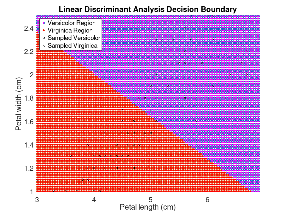
Train a linear discriminant classifier for Gamma = 0.5 and plot the decision boundaries.
 load fisheriris
 idx = ! strcmp (species, 'setosa');
 X = meas(idx,3:4);
 Y = cast (strcmpi (species(idx), 'virginica'), 'double');
 obj = fitcdiscr (X, Y, 'Gamma', 0.5)
obj =

  ClassificationDiscriminant

             ResponseName: 'Y'
               ClassNames: [0 1]
           ScoreTransform: 'none'
          NumObservations: 100
            NumPredictors: 2
              DiscrimType: 'linear'
                       Mu: [2x2 double]
                   Coeffs: [2x2 struct]
 x1 = [min(X(:,1)):0.03:max(X(:,1))];
 x2 = [min(X(:,2)):0.02:max(X(:,2))];
 [x1G, x2G] = meshgrid (x1, x2);
 XGrid = [x1G(:), x2G(:)];
 pred = predict (obj, XGrid);
 gidx = logical (pred);
 figure
 scatter (XGrid(gidx,1), XGrid(gidx,2), 'markerfacecolor', 'magenta');
 hold on
 scatter (XGrid(! gidx,1), XGrid(! gidx,2), 'markerfacecolor', 'red');
 plot (X(Y == 0, 1), X(Y == 0, 2), 'ko', X(Y == 1, 1), X(Y == 1, 2), 'kx');
 xlabel ('Petal length (cm)');
 ylabel ('Petal width (cm)');
 title ('Linear Discriminant Analysis Decision Boundary');
 legend ({'Versicolor Region', 'Virginica Region', ...
         'Sampled Versicolor', 'Sampled Virginica'}, ...
         'location', 'northwest')
 axis tight
 hold off
Fit from a table, and predict on one
 load fisheriris
 T = table (meas(:,1), meas(:,2), meas(:,3), meas(:,4), ...
            'VariableNames', {'SL', 'SW', 'PL', 'PW'});
 T.Species = categorical (species);
A model formula names the response and the predictors together, and holds main effects only
 Mdl = fitcdiscr (T, 'Species ~ PL + PW');
 Mdl.PredictorNames
ans =
  1x2 cell array

    {'PL'}    {'PW'}
Mdl.ResponseName
ans = Species
predict matches the table's variables by name, so a column the model was not fitted on is passed over
 label = predict (Mdl, T(1:5,:));
 label'
ans =
  1x5 categorical array

    setosa    setosa    setosa    setosa    setosa