Categories &
Functions List
- BetaDistribution
- BinomialDistribution
- BirnbaumSaundersDistribution
- BurrDistribution
- ExponentialDistribution
- ExtremeValueDistribution
- GammaDistribution
- GeneralizedExtremeValueDistribution
- GeneralizedParetoDistribution
- HalfNormalDistribution
- InverseGaussianDistribution
- LogisticDistribution
- LoglogisticDistribution
- LognormalDistribution
- LoguniformDistribution
- MultinomialDistribution
- NakagamiDistribution
- NegativeBinomialDistribution
- NormalDistribution
- PiecewiseLinearDistribution
- PoissonDistribution
- RayleighDistribution
- RicianDistribution
- tLocationScaleDistribution
- TriangularDistribution
- UniformDistribution
- WeibullDistribution
- betafit
- betalike
- binofit
- binolike
- bisafit
- bisalike
- burrfit
- burrlike
- evfit
- evlike
- expfit
- explike
- gamfit
- gamlike
- geofit
- gevfit_lmom
- gevfit
- gevlike
- gpfit
- gplike
- gumbelfit
- gumbellike
- hnfit
- hnlike
- invgfit
- invglike
- logifit
- logilike
- loglfit
- logllike
- lognfit
- lognlike
- nakafit
- nakalike
- nbinfit
- nbinlike
- normfit
- normlike
- poissfit
- poisslike
- raylfit
- rayllike
- ricefit
- ricelike
- tlsfit
- tlslike
- unidfit
- unifit
- wblfit
- wbllike
- betacdf
- betainv
- betapdf
- betarnd
- binocdf
- binoinv
- binopdf
- binornd
- bisacdf
- bisainv
- bisapdf
- bisarnd
- burrcdf
- burrinv
- burrpdf
- burrrnd
- bvncdf
- bvtcdf
- cauchycdf
- cauchyinv
- cauchypdf
- cauchyrnd
- chi2cdf
- chi2inv
- chi2pdf
- chi2rnd
- copulacdf
- copulapdf
- copularnd
- evcdf
- evinv
- evpdf
- evrnd
- expcdf
- expinv
- exppdf
- exprnd
- fcdf
- finv
- fpdf
- frnd
- gamcdf
- gaminv
- gampdf
- gamrnd
- geocdf
- geoinv
- geopdf
- geornd
- gevcdf
- gevinv
- gevpdf
- gevrnd
- gpcdf
- gpinv
- gppdf
- gprnd
- gumbelcdf
- gumbelinv
- gumbelpdf
- gumbelrnd
- hncdf
- hninv
- hnpdf
- hnrnd
- hygecdf
- hygeinv
- hygepdf
- hygernd
- invgcdf
- invginv
- invgpdf
- invgrnd
- iwishpdf
- iwishrnd
- jsucdf
- jsupdf
- laplacecdf
- laplaceinv
- laplacepdf
- laplacernd
- logicdf
- logiinv
- logipdf
- logirnd
- loglcdf
- loglinv
- loglpdf
- loglrnd
- logncdf
- logninv
- lognpdf
- lognrnd
- mnpdf
- mnrnd
- mvncdf
- mvnpdf
- mvnrnd
- mvtcdf
- mvtpdf
- mvtrnd
- mvtcdfqmc
- nakacdf
- nakainv
- nakapdf
- nakarnd
- nbincdf
- nbininv
- nbinpdf
- nbinrnd
- ncfcdf
- ncfinv
- ncfpdf
- ncfrnd
- nctcdf
- nctinv
- nctpdf
- nctrnd
- ncx2cdf
- ncx2inv
- ncx2pdf
- ncx2rnd
- normcdf
- norminv
- normpdf
- normrnd
- plcdf
- plinv
- plpdf
- plrnd
- poisscdf
- poissinv
- poisspdf
- poissrnd
- raylcdf
- raylinv
- raylpdf
- raylrnd
- ricecdf
- riceinv
- ricepdf
- ricernd
- tcdf
- tinv
- tpdf
- trnd
- tlscdf
- tlsinv
- tlspdf
- tlsrnd
- tricdf
- triinv
- tripdf
- trirnd
- unidcdf
- unidinv
- unidpdf
- unidrnd
- unifcdf
- unifinv
- unifpdf
- unifrnd
- vmcdf
- vminv
- vmpdf
- vmrnd
- wblcdf
- wblinv
- wblpdf
- wblrnd
- wienrnd
- wishpdf
- wishrnd
- adtest
- anova
- anova1
- anova2
- anovan
- bartlett_test
- barttest
- binotest
- chi2gof
- chi2test
- correlation_test
- fishertest
- friedman
- hotelling_t2test
- hotelling_t2test2
- kruskalwallis
- kstest
- kstest2
- levene_test
- manova1
- mcnemar_test
- multcompare
- ranksum
- regression_ftest
- regression_ttest
- runstest
- sampsizepwr
- signrank
- signtest
- tiedrank
- ttest
- ttest2
- vartest
- vartest2
- vartestn
- ztest
- ztest2
Function Reference: loglcdf
statistics: p = loglcdf (x, mu, sigma)
statistics: p = loglcdf (x, mu, sigma,
'upper')
Loglogistic cumulative distribution function (CDF).
For each element of x, compute the cumulative distribution function (CDF) of the loglogistic distribution with mean parameter mu and scale parameter sigma. The size of p is the common size of x, mu, and sigma. A scalar input functions as a constant matrix of the same size as the other inputs.
Mean of logarithmic values mu must be a non-negative real value, scale
parameter of logarithmic values sigma must be a positive real value and
x is supported in the range , otherwise NaN is
returned.
p = loglcdf (x, mu, sigma, "upper") computes
the upper tail probability of the log-logistic distribution with parameters
mu and sigma, at the values in x.
Further information about the loglogistic distribution can be found at https://en.wikipedia.org/wiki/Log-logistic_distribution
OCTAVE/MATLAB use an alternative parameterization given by the pair , i.e. mu and sigma, in analogy with the logistic distribution. Their relation to the and parameters used in Wikipedia are given below:
-
mu = log (a) -
sigma = 1 / a
See also: loglinv, loglpdf, loglrnd, loglfit, logllike, loglstat
Source Code: loglcdf
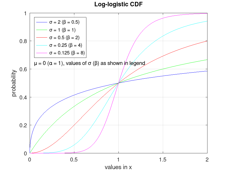
Example: 1
Plot various CDFs from the log-logistic distribution
 x = 0:0.001:2;
 p1 = loglcdf (x, log (1), 1/0.5);
 p2 = loglcdf (x, log (1), 1);
 p3 = loglcdf (x, log (1), 1/2);
 p4 = loglcdf (x, log (1), 1/4);
 p5 = loglcdf (x, log (1), 1/8);
 plot (x, p1, '-b', x, p2, '-g', x, p3, '-r', x, p4, '-c', x, p5, '-m')
 legend ({'σ = 2 (β = 0.5)', 'σ = 1 (β = 1)', 'σ = 0.5 (β = 2)', ...
          'σ = 0.25 (β = 4)', 'σ = 0.125 (β = 8)'}, 'location', 'northwest')
 grid on
 title ('Log-logistic CDF')
 xlabel ('values in x')
 ylabel ('probability')
 text (0.05, 0.64, 'μ = 0 (α = 1), values of σ (β) as shown in legend')