Statistics: RegressionGAM

Class Definition: `RegressionGAM`

statistics: RegressionGAM

Generalized additive model for regression.

A RegressionGAM object holds a generalized additive model fitted to a continuous response, and predicts the response for new data with the predict method. The model is a sum of one shape function per predictor, and optionally one per pair of predictors, each learned from the data rather than assumed.

Two engines fit it. 'boostedtrees', the default, boosts shallow decision trees one predictor at a time; 'splines' boosts smoothing splines. The properties describing the engine that was not used are empty.

The object keeps its training data, which resubPredict, resubLoss and crossval work on; compact drops it and returns a CompactRegressionGAM, which still predicts.

Create a RegressionGAM object with fitrgam or the class constructor.

Source Code: RegressionGAM

The RegressionGAM class contains the following properties:

A numeric matrix with one row per observation and one column per predictor of the training data. This property is read-only.

Where the model was fitted from a table, the predictors are the coded matrix and not the table: a variable holding levels is stored as its level codes, and the coding is kept with the model.

Train a RegressionGAM Model for synthetic values

 rng (42);
 f1 = @(x) cos (3 * x);
 f2 = @(x) x .^ 3;
 x1 = 2 * rand (50, 1) - 1;
 x2 = 2 * rand (50, 1) - 1;
 y = f1(x1) + f2(x2);
 y = y + y .* 0.2 .* rand (50,1);
 X = [x1, x2];
 a = fitrgam (X, y)

a =

  RegressionGAM

             ResponseName: 'Y'
          NumObservations: 50
            NumPredictors: 2
        ResponseTransform: 'none'
                Intercept: 0.0671178
                    Knots: []
                    Order: []
                      Tol:

Declare two different functions

 rng (42);
 f1 = @(x) cos (3 * x);
 f2 = @(x) x .^ 3;

Generate 80 samples for f1 and f2

 x = [-4*pi:0.1*pi:4*pi-0.1*pi]';
 X1 = f1(x);
 X2 = f2(x);

Create a synthetic response by adding noise

 Ytrue = X1 + X2;
 Y = Ytrue + Ytrue .* 0.2 .* rand (80,1);

Assemble predictor data

 X = [X1, X2];

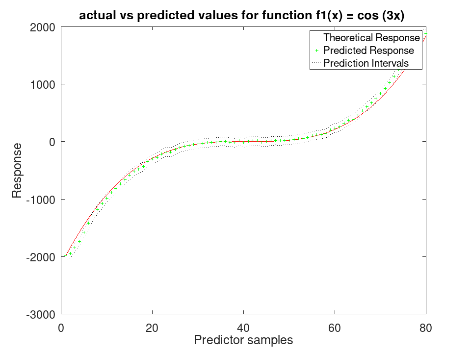
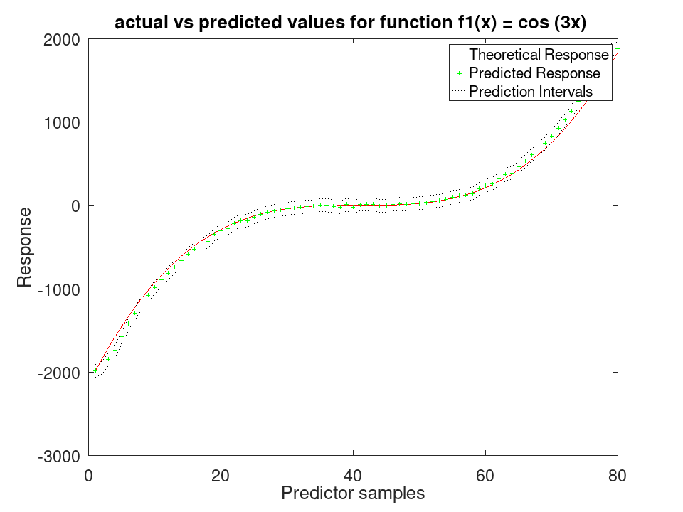
Train the GAM and test on the same data A standard deviation and a prediction interval come from the spline engine, which fits one; the boosted-tree engine reports none.

 a = fitrgam (X, Y, 'FitMethod', 'splines', 'order', [5, 5]);
 [ypred, ySDsd, yInt] = predict (a, X);

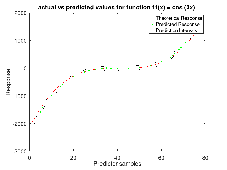
Plot the results

 figure
 [sortedY, indY] = sort (Ytrue);
 plot (sortedY, 'r-');
 xlim ([0, 80]);
 hold on
 plot (ypred(indY), 'g+')
 plot (yInt(indY,1), 'k:')
 plot (yInt(indY,2), 'k:')
 xlabel ('Predictor samples');
 ylabel ('Response');
 title ('actual vs predicted values for function f1(x) = cos (3x) ');
 legend ({'Theoretical Response', 'Predicted Response', 'Prediction Intervals'});

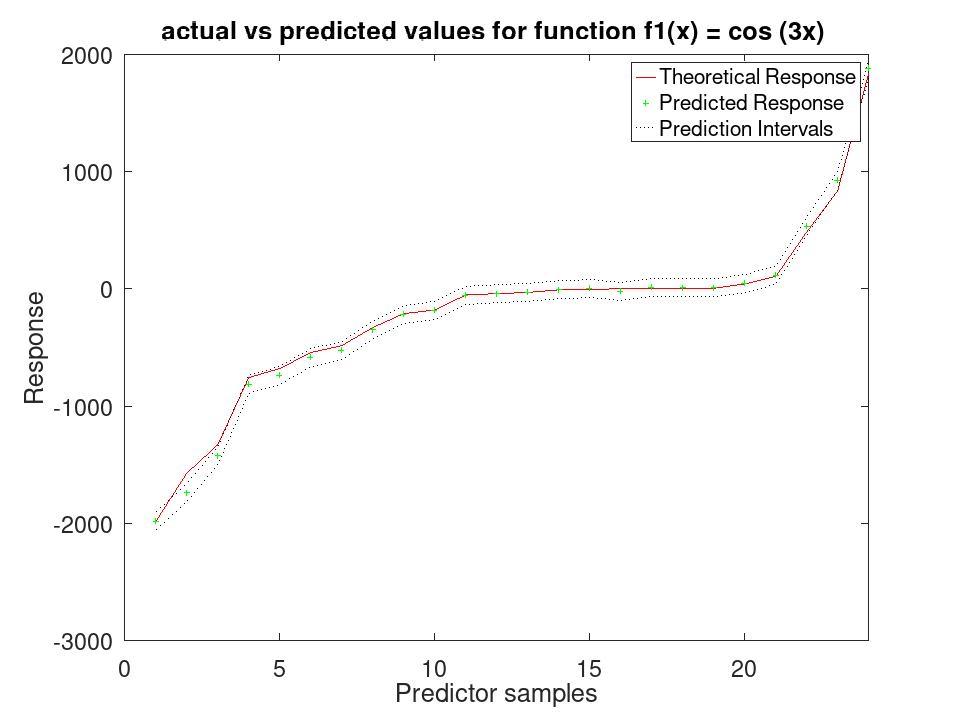
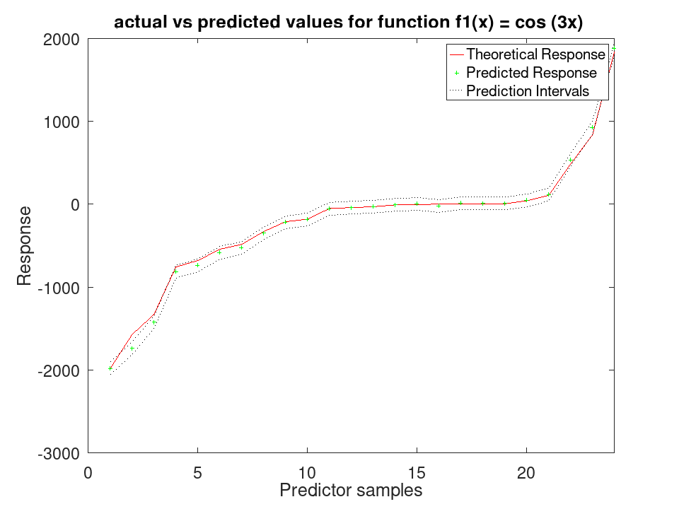
Use 30% Holdout partitioning for training and testing data

 C = cvpartition (80, 'HoldOut', 0.3);
 [ypred, ySDsd, yInt] = predict (a, X(test (C),:));

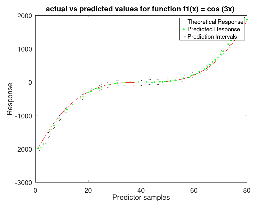
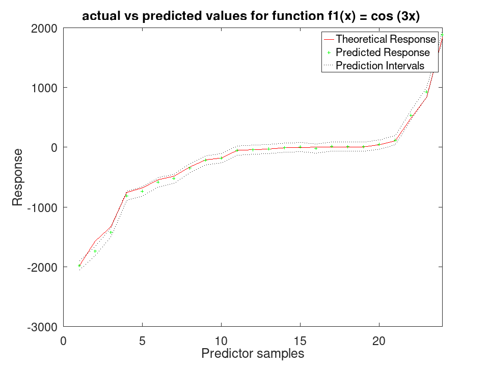
Plot the results

 figure
 [sortedY, indY] = sort (Ytrue(test (C)));
 plot (sortedY, 'r-');
 xlim ([0, sum(test(C))]);
 hold on
 plot (ypred(indY), 'g+')
 plot (yInt(indY,1),'k:')
 plot (yInt(indY,2),'k:')
 xlabel ('Predictor samples');
 ylabel ('Response');
 title ('actual vs predicted values for function f1(x) = cos (3x) ');
 legend ({'Theoretical Response', 'Predicted Response', 'Prediction Intervals'});

A numeric column vector with one entry per observation of the training data. This property is read-only.

Train a RegressionGAM Model for synthetic values

 rng (42);
 f1 = @(x) cos (3 * x);
 f2 = @(x) x .^ 3;
 x1 = 2 * rand (50, 1) - 1;
 x2 = 2 * rand (50, 1) - 1;
 y = f1(x1) + f2(x2);
 y = y + y .* 0.2 .* rand (50,1);
 X = [x1, x2];
 a = fitrgam (X, y)

a =

  RegressionGAM

             ResponseName: 'Y'
          NumObservations: 50
            NumPredictors: 2
        ResponseTransform: 'none'
                Intercept: 0.0671178
                    Knots: []
                    Order: []
                      Tol:

Declare two different functions

 rng (42);
 f1 = @(x) cos (3 * x);
 f2 = @(x) x .^ 3;

Generate 80 samples for f1 and f2

 x = [-4*pi:0.1*pi:4*pi-0.1*pi]';
 X1 = f1(x);
 X2 = f2(x);

Create a synthetic response by adding noise

 Ytrue = X1 + X2;
 Y = Ytrue + Ytrue .* 0.2 .* rand (80,1);

Assemble predictor data

 X = [X1, X2];

Train the GAM and test on the same data A standard deviation and a prediction interval come from the spline engine, which fits one; the boosted-tree engine reports none.

 a = fitrgam (X, Y, 'FitMethod', 'splines', 'order', [5, 5]);
 [ypred, ySDsd, yInt] = predict (a, X);

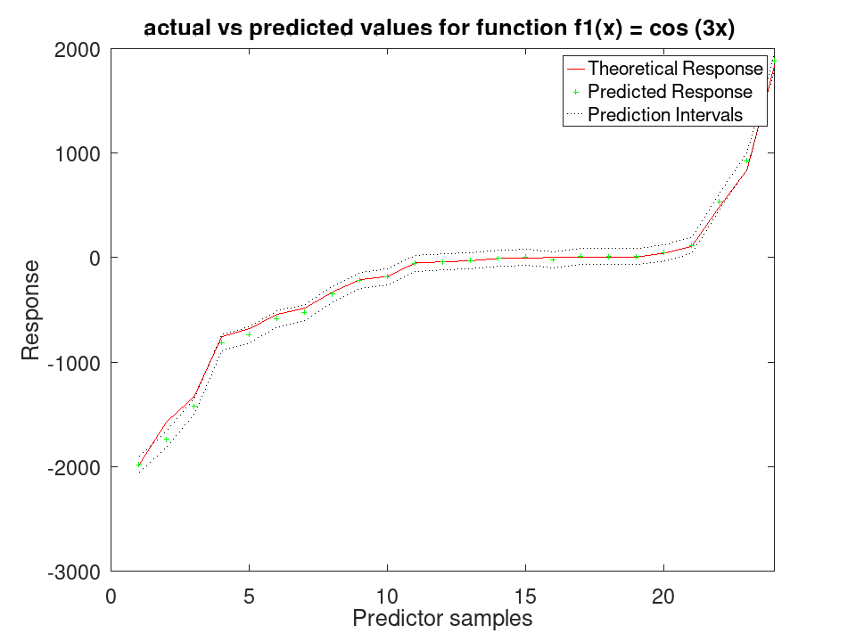
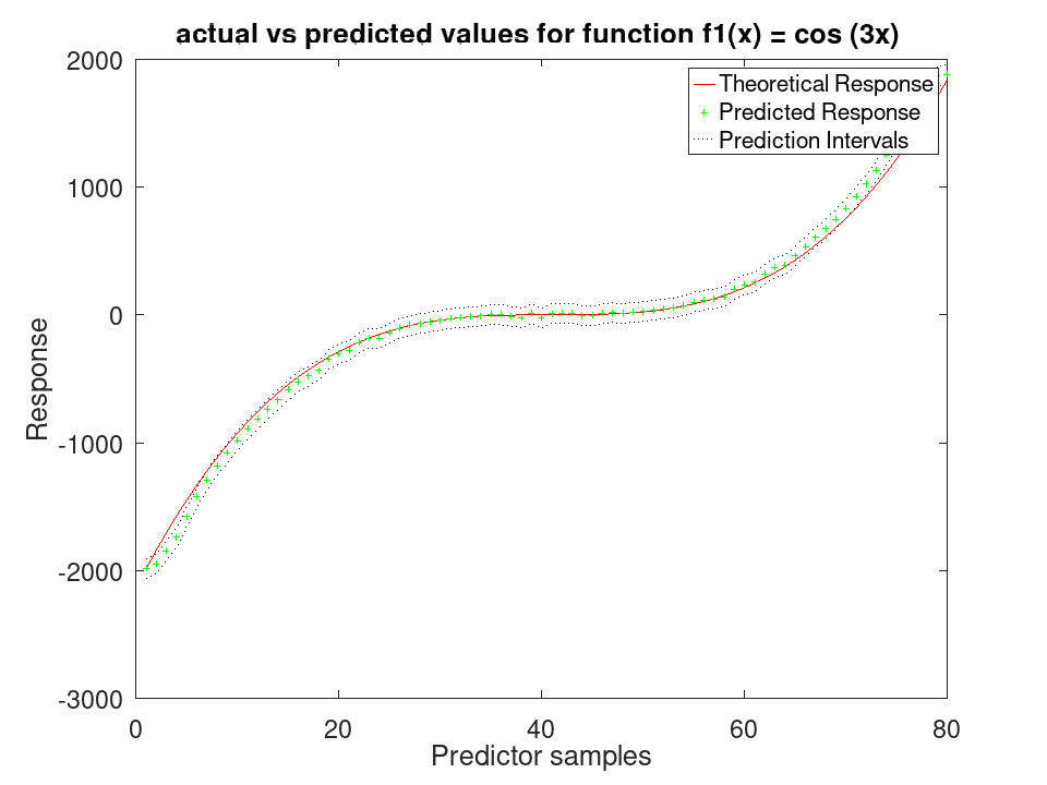
Plot the results

 figure
 [sortedY, indY] = sort (Ytrue);
 plot (sortedY, 'r-');
 xlim ([0, 80]);
 hold on
 plot (ypred(indY), 'g+')
 plot (yInt(indY,1), 'k:')
 plot (yInt(indY,2), 'k:')
 xlabel ('Predictor samples');
 ylabel ('Response');
 title ('actual vs predicted values for function f1(x) = cos (3x) ');
 legend ({'Theoretical Response', 'Predicted Response', 'Prediction Intervals'});

Use 30% Holdout partitioning for training and testing data

 C = cvpartition (80, 'HoldOut', 0.3);
 [ypred, ySDsd, yInt] = predict (a, X(test (C),:));

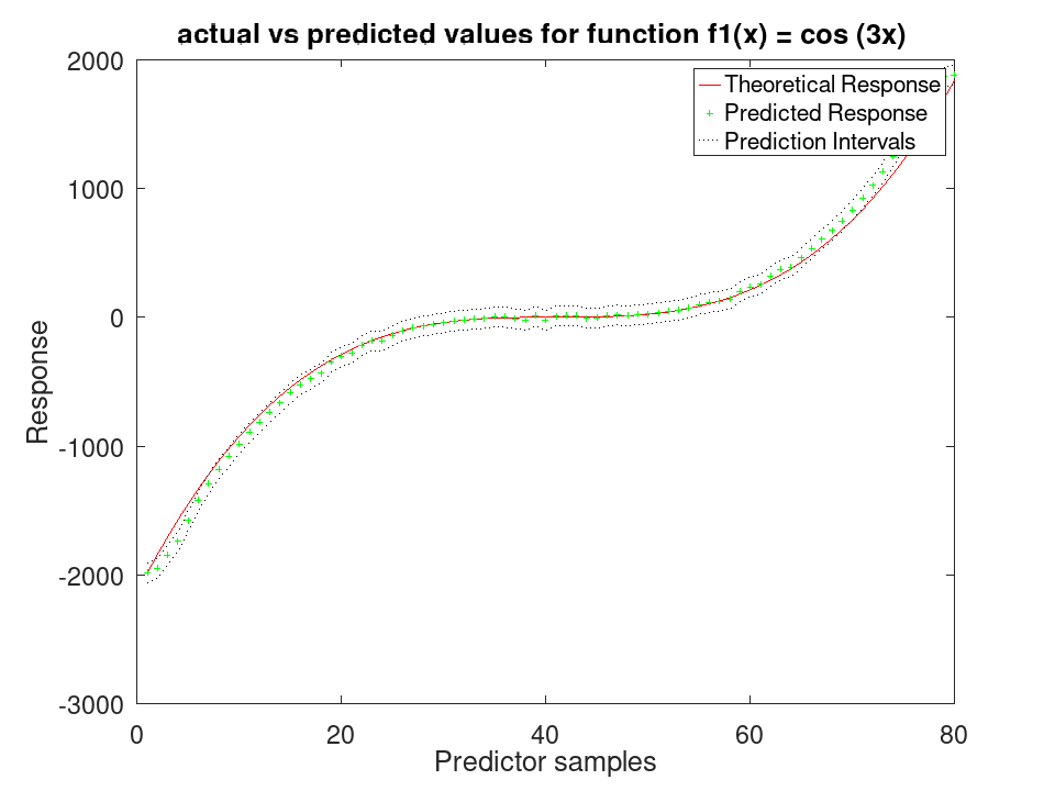
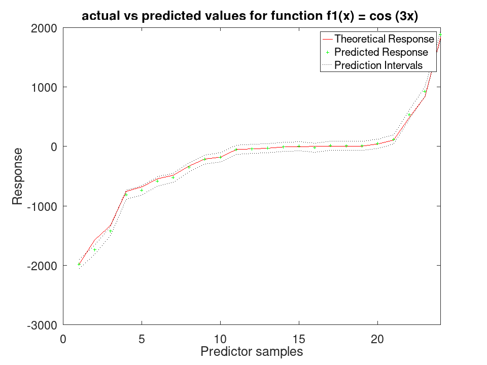
Plot the results

 figure
 [sortedY, indY] = sort (Ytrue(test (C)));
 plot (sortedY, 'r-');
 xlim ([0, sum(test(C))]);
 hold on
 plot (ypred(indY), 'g+')
 plot (yInt(indY,1),'k:')
 plot (yInt(indY,2),'k:')
 xlabel ('Predictor samples');
 ylabel ('Response');
 title ('actual vs predicted values for function f1(x) = cos (3x) ');
 legend ({'Theoretical Response', 'Predicted Response', 'Prediction Intervals'});

A positive integer, the number of observations of the training data the model was fitted on, rows with a missing response excluded. This property is read-only.

Train a RegressionGAM Model for synthetic values

 rng (42);
 f1 = @(x) cos (3 * x);
 f2 = @(x) x .^ 3;
 x1 = 2 * rand (50, 1) - 1;
 x2 = 2 * rand (50, 1) - 1;
 y = f1(x1) + f2(x2);
 y = y + y .* 0.2 .* rand (50,1);
 X = [x1, x2];
 a = fitrgam (X, y)

a =

  RegressionGAM

             ResponseName: 'Y'
          NumObservations: 50
            NumPredictors: 2
        ResponseTransform: 'none'
                Intercept: 0.0671178
                    Knots: []
                    Order: []
                      Tol:

Declare two different functions

 rng (42);
 f1 = @(x) cos (3 * x);
 f2 = @(x) x .^ 3;

Generate 80 samples for f1 and f2

 x = [-4*pi:0.1*pi:4*pi-0.1*pi]';
 X1 = f1(x);
 X2 = f2(x);

Create a synthetic response by adding noise

 Ytrue = X1 + X2;
 Y = Ytrue + Ytrue .* 0.2 .* rand (80,1);

Assemble predictor data

 X = [X1, X2];

Train the GAM and test on the same data A standard deviation and a prediction interval come from the spline engine, which fits one; the boosted-tree engine reports none.

 a = fitrgam (X, Y, 'FitMethod', 'splines', 'order', [5, 5]);
 [ypred, ySDsd, yInt] = predict (a, X);

Plot the results

 figure
 [sortedY, indY] = sort (Ytrue);
 plot (sortedY, 'r-');
 xlim ([0, 80]);
 hold on
 plot (ypred(indY), 'g+')
 plot (yInt(indY,1), 'k:')
 plot (yInt(indY,2), 'k:')
 xlabel ('Predictor samples');
 ylabel ('Response');
 title ('actual vs predicted values for function f1(x) = cos (3x) ');
 legend ({'Theoretical Response', 'Predicted Response', 'Prediction Intervals'});

Use 30% Holdout partitioning for training and testing data

 C = cvpartition (80, 'HoldOut', 0.3);
 [ypred, ySDsd, yInt] = predict (a, X(test (C),:));

Plot the results

 figure
 [sortedY, indY] = sort (Ytrue(test (C)));
 plot (sortedY, 'r-');
 xlim ([0, sum(test(C))]);
 hold on
 plot (ypred(indY), 'g+')
 plot (yInt(indY,1),'k:')
 plot (yInt(indY,2),'k:')
 xlabel ('Predictor samples');
 ylabel ('Response');
 title ('actual vs predicted values for function f1(x) = cos (3x) ');
 legend ({'Theoretical Response', 'Predicted Response', 'Prediction Intervals'});

A logical column vector with the same length as the observations in the original predictor data X, true for each row that was used for fitting the RegressionGAM model. It is empty, [], when every observation was used, so a non-empty value means that rows holding missing values were dropped. This property is read-only.

Train a RegressionGAM Model for synthetic values

 rng (42);
 f1 = @(x) cos (3 * x);
 f2 = @(x) x .^ 3;
 x1 = 2 * rand (50, 1) - 1;
 x2 = 2 * rand (50, 1) - 1;
 y = f1(x1) + f2(x2);
 y = y + y .* 0.2 .* rand (50,1);
 X = [x1, x2];
 a = fitrgam (X, y)

a =

  RegressionGAM

             ResponseName: 'Y'
          NumObservations: 50
            NumPredictors: 2
        ResponseTransform: 'none'
                Intercept: 0.0671178
                    Knots: []
                    Order: []
                      Tol:

Declare two different functions

 rng (42);
 f1 = @(x) cos (3 * x);
 f2 = @(x) x .^ 3;

Generate 80 samples for f1 and f2

 x = [-4*pi:0.1*pi:4*pi-0.1*pi]';
 X1 = f1(x);
 X2 = f2(x);

Create a synthetic response by adding noise

 Ytrue = X1 + X2;
 Y = Ytrue + Ytrue .* 0.2 .* rand (80,1);

Assemble predictor data

 X = [X1, X2];

Train the GAM and test on the same data A standard deviation and a prediction interval come from the spline engine, which fits one; the boosted-tree engine reports none.

 a = fitrgam (X, Y, 'FitMethod', 'splines', 'order', [5, 5]);
 [ypred, ySDsd, yInt] = predict (a, X);

Plot the results

 figure
 [sortedY, indY] = sort (Ytrue);
 plot (sortedY, 'r-');
 xlim ([0, 80]);
 hold on
 plot (ypred(indY), 'g+')
 plot (yInt(indY,1), 'k:')
 plot (yInt(indY,2), 'k:')
 xlabel ('Predictor samples');
 ylabel ('Response');
 title ('actual vs predicted values for function f1(x) = cos (3x) ');
 legend ({'Theoretical Response', 'Predicted Response', 'Prediction Intervals'});

Use 30% Holdout partitioning for training and testing data

 C = cvpartition (80, 'HoldOut', 0.3);
 [ypred, ySDsd, yInt] = predict (a, X(test (C),:));

Plot the results

 figure
 [sortedY, indY] = sort (Ytrue(test (C)));
 plot (sortedY, 'r-');
 xlim ([0, sum(test(C))]);
 hold on
 plot (ypred(indY), 'g+')
 plot (yInt(indY,1),'k:')
 plot (yInt(indY,2),'k:')
 xlabel ('Predictor samples');
 ylabel ('Response');
 title ('actual vs predicted values for function f1(x) = cos (3x) ');
 legend ({'Theoretical Response', 'Predicted Response', 'Prediction Intervals'});

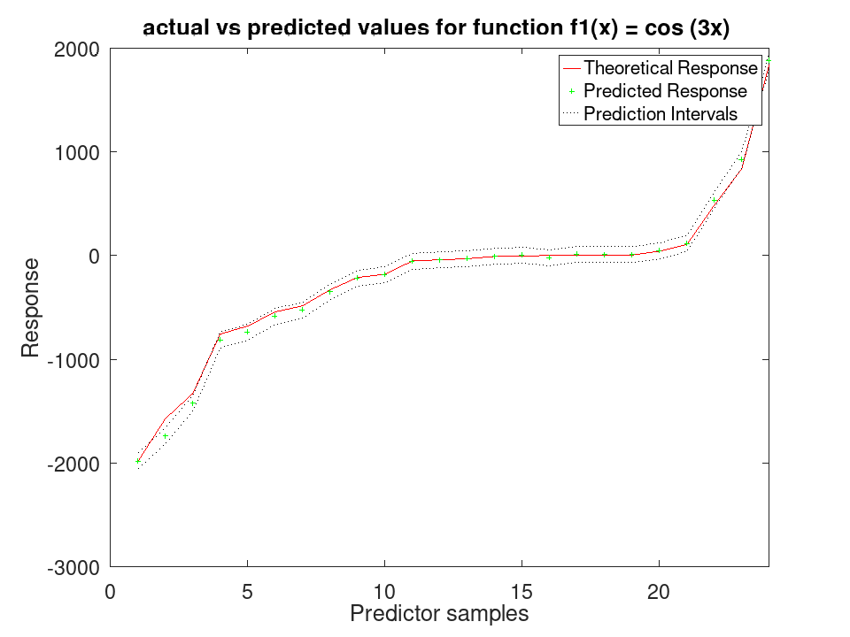
A positive integer, the number of predictors of the training data. This property is read-only.

Train a RegressionGAM Model for synthetic values

 rng (42);
 f1 = @(x) cos (3 * x);
 f2 = @(x) x .^ 3;
 x1 = 2 * rand (50, 1) - 1;
 x2 = 2 * rand (50, 1) - 1;
 y = f1(x1) + f2(x2);
 y = y + y .* 0.2 .* rand (50,1);
 X = [x1, x2];
 a = fitrgam (X, y)

a =

  RegressionGAM

             ResponseName: 'Y'
          NumObservations: 50
            NumPredictors: 2
        ResponseTransform: 'none'
                Intercept: 0.0671178
                    Knots: []
                    Order: []
                      Tol:

Declare two different functions

 rng (42);
 f1 = @(x) cos (3 * x);
 f2 = @(x) x .^ 3;

Generate 80 samples for f1 and f2

 x = [-4*pi:0.1*pi:4*pi-0.1*pi]';
 X1 = f1(x);
 X2 = f2(x);

Create a synthetic response by adding noise

 Ytrue = X1 + X2;
 Y = Ytrue + Ytrue .* 0.2 .* rand (80,1);

Assemble predictor data

 X = [X1, X2];

Train the GAM and test on the same data A standard deviation and a prediction interval come from the spline engine, which fits one; the boosted-tree engine reports none.

 a = fitrgam (X, Y, 'FitMethod', 'splines', 'order', [5, 5]);
 [ypred, ySDsd, yInt] = predict (a, X);

Plot the results

 figure
 [sortedY, indY] = sort (Ytrue);
 plot (sortedY, 'r-');
 xlim ([0, 80]);
 hold on
 plot (ypred(indY), 'g+')
 plot (yInt(indY,1), 'k:')
 plot (yInt(indY,2), 'k:')
 xlabel ('Predictor samples');
 ylabel ('Response');
 title ('actual vs predicted values for function f1(x) = cos (3x) ');
 legend ({'Theoretical Response', 'Predicted Response', 'Prediction Intervals'});

Use 30% Holdout partitioning for training and testing data

 C = cvpartition (80, 'HoldOut', 0.3);
 [ypred, ySDsd, yInt] = predict (a, X(test (C),:));

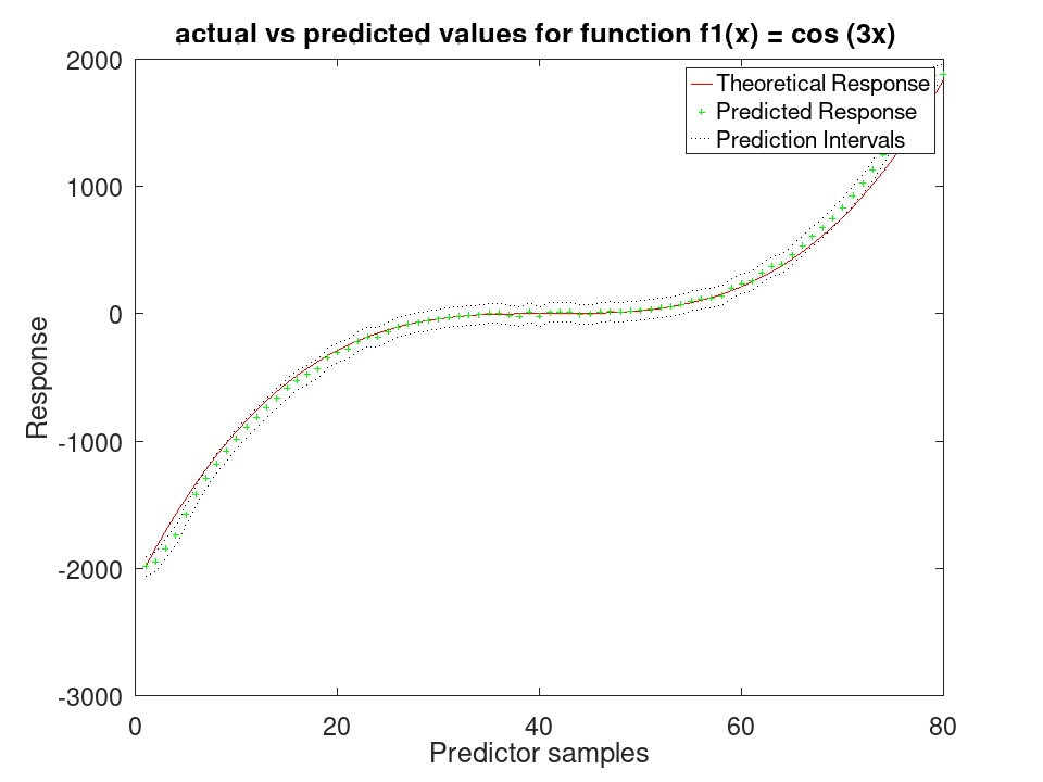
Plot the results

 figure
 [sortedY, indY] = sort (Ytrue(test (C)));
 plot (sortedY, 'r-');
 xlim ([0, sum(test(C))]);
 hold on
 plot (ypred(indY), 'g+')
 plot (yInt(indY,1),'k:')
 plot (yInt(indY,2),'k:')
 xlabel ('Predictor samples');
 ylabel ('Response');
 title ('actual vs predicted values for function f1(x) = cos (3x) ');
 legend ({'Theoretical Response', 'Predicted Response', 'Prediction Intervals'});

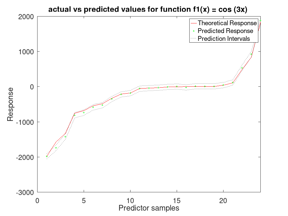
A cell array of character vectors naming the predictors, in the order they appear in the training data. This property is read-only.

Train a RegressionGAM Model for synthetic values

 rng (42);
 f1 = @(x) cos (3 * x);
 f2 = @(x) x .^ 3;
 x1 = 2 * rand (50, 1) - 1;
 x2 = 2 * rand (50, 1) - 1;
 y = f1(x1) + f2(x2);
 y = y + y .* 0.2 .* rand (50,1);
 X = [x1, x2];
 a = fitrgam (X, y)

a =

  RegressionGAM

             ResponseName: 'Y'
          NumObservations: 50
            NumPredictors: 2
        ResponseTransform: 'none'
                Intercept: 0.0671178
                    Knots: []
                    Order: []
                      Tol:

Declare two different functions

 rng (42);
 f1 = @(x) cos (3 * x);
 f2 = @(x) x .^ 3;

Generate 80 samples for f1 and f2

 x = [-4*pi:0.1*pi:4*pi-0.1*pi]';
 X1 = f1(x);
 X2 = f2(x);

Create a synthetic response by adding noise

 Ytrue = X1 + X2;
 Y = Ytrue + Ytrue .* 0.2 .* rand (80,1);

Assemble predictor data

 X = [X1, X2];

Train the GAM and test on the same data A standard deviation and a prediction interval come from the spline engine, which fits one; the boosted-tree engine reports none.

 a = fitrgam (X, Y, 'FitMethod', 'splines', 'order', [5, 5]);
 [ypred, ySDsd, yInt] = predict (a, X);

Plot the results

 figure
 [sortedY, indY] = sort (Ytrue);
 plot (sortedY, 'r-');
 xlim ([0, 80]);
 hold on
 plot (ypred(indY), 'g+')
 plot (yInt(indY,1), 'k:')
 plot (yInt(indY,2), 'k:')
 xlabel ('Predictor samples');
 ylabel ('Response');
 title ('actual vs predicted values for function f1(x) = cos (3x) ');
 legend ({'Theoretical Response', 'Predicted Response', 'Prediction Intervals'});

Use 30% Holdout partitioning for training and testing data

 C = cvpartition (80, 'HoldOut', 0.3);
 [ypred, ySDsd, yInt] = predict (a, X(test (C),:));

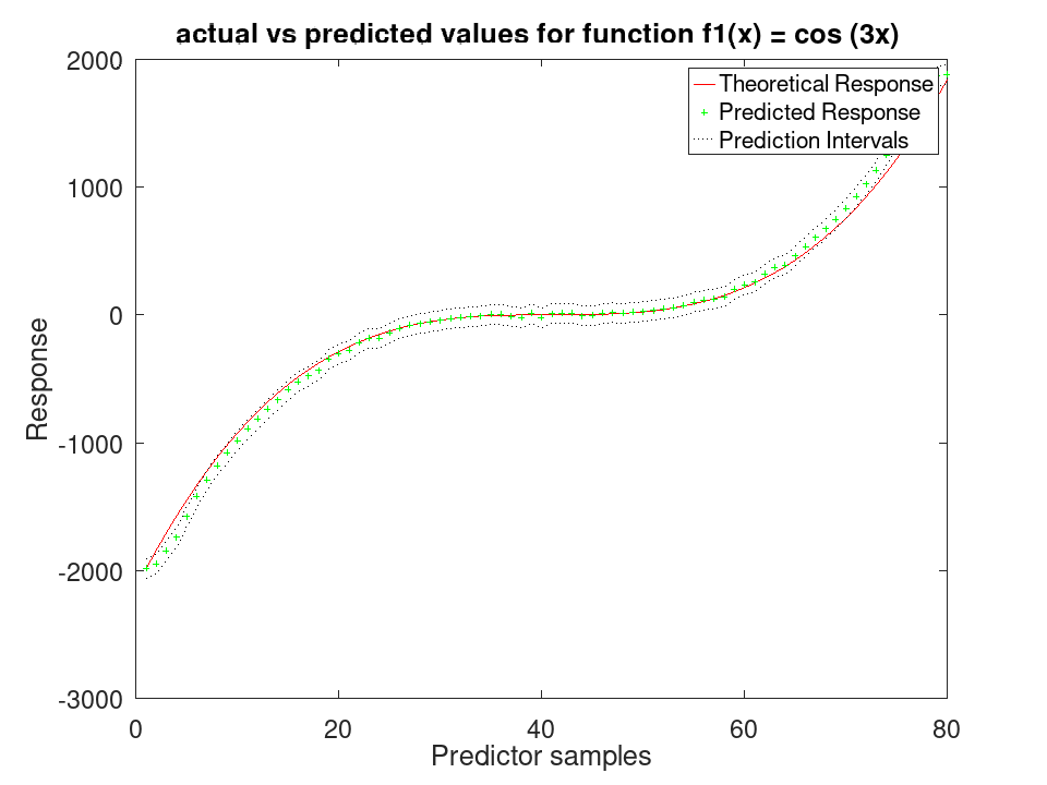
Plot the results

 figure
 [sortedY, indY] = sort (Ytrue(test (C)));
 plot (sortedY, 'r-');
 xlim ([0, sum(test(C))]);
 hold on
 plot (ypred(indY), 'g+')
 plot (yInt(indY,1),'k:')
 plot (yInt(indY,2),'k:')
 xlabel ('Predictor samples');
 ylabel ('Response');
 title ('actual vs predicted values for function f1(x) = cos (3x) ');
 legend ({'Theoretical Response', 'Predicted Response', 'Prediction Intervals'});

A character vector naming the response variable Y. This property is read-only.

Train a RegressionGAM Model for synthetic values

 rng (42);
 f1 = @(x) cos (3 * x);
 f2 = @(x) x .^ 3;
 x1 = 2 * rand (50, 1) - 1;
 x2 = 2 * rand (50, 1) - 1;
 y = f1(x1) + f2(x2);
 y = y + y .* 0.2 .* rand (50,1);
 X = [x1, x2];
 a = fitrgam (X, y)

a =

  RegressionGAM

             ResponseName: 'Y'
          NumObservations: 50
            NumPredictors: 2
        ResponseTransform: 'none'
                Intercept: 0.0671178
                    Knots: []
                    Order: []
                      Tol:

Declare two different functions

 rng (42);
 f1 = @(x) cos (3 * x);
 f2 = @(x) x .^ 3;

Generate 80 samples for f1 and f2

 x = [-4*pi:0.1*pi:4*pi-0.1*pi]';
 X1 = f1(x);
 X2 = f2(x);

Create a synthetic response by adding noise

 Ytrue = X1 + X2;
 Y = Ytrue + Ytrue .* 0.2 .* rand (80,1);

Assemble predictor data

 X = [X1, X2];

Train the GAM and test on the same data A standard deviation and a prediction interval come from the spline engine, which fits one; the boosted-tree engine reports none.

 a = fitrgam (X, Y, 'FitMethod', 'splines', 'order', [5, 5]);
 [ypred, ySDsd, yInt] = predict (a, X);

Plot the results

 figure
 [sortedY, indY] = sort (Ytrue);
 plot (sortedY, 'r-');
 xlim ([0, 80]);
 hold on
 plot (ypred(indY), 'g+')
 plot (yInt(indY,1), 'k:')
 plot (yInt(indY,2), 'k:')
 xlabel ('Predictor samples');
 ylabel ('Response');
 title ('actual vs predicted values for function f1(x) = cos (3x) ');
 legend ({'Theoretical Response', 'Predicted Response', 'Prediction Intervals'});

Use 30% Holdout partitioning for training and testing data

 C = cvpartition (80, 'HoldOut', 0.3);
 [ypred, ySDsd, yInt] = predict (a, X(test (C),:));

Plot the results

 figure
 [sortedY, indY] = sort (Ytrue(test (C)));
 plot (sortedY, 'r-');
 xlim ([0, sum(test(C))]);
 hold on
 plot (ypred(indY), 'g+')
 plot (yInt(indY,1),'k:')
 plot (yInt(indY,2),'k:')
 xlabel ('Predictor samples');
 ylabel ('Response');
 title ('actual vs predicted values for function f1(x) = cos (3x) ');
 legend ({'Theoretical Response', 'Predicted Response', 'Prediction Intervals'});

A numeric vector holding the column of each predictor treated as categorical, and empty when none is. This property is read-only.

Train a RegressionGAM Model for synthetic values

 rng (42);
 f1 = @(x) cos (3 * x);
 f2 = @(x) x .^ 3;
 x1 = 2 * rand (50, 1) - 1;
 x2 = 2 * rand (50, 1) - 1;
 y = f1(x1) + f2(x2);
 y = y + y .* 0.2 .* rand (50,1);
 X = [x1, x2];
 a = fitrgam (X, y)

a =

  RegressionGAM

             ResponseName: 'Y'
          NumObservations: 50
            NumPredictors: 2
        ResponseTransform: 'none'
                Intercept: 0.0671178
                    Knots: []
                    Order: []
                      Tol:

Declare two different functions

 rng (42);
 f1 = @(x) cos (3 * x);
 f2 = @(x) x .^ 3;

Generate 80 samples for f1 and f2

 x = [-4*pi:0.1*pi:4*pi-0.1*pi]';
 X1 = f1(x);
 X2 = f2(x);

Create a synthetic response by adding noise

 Ytrue = X1 + X2;
 Y = Ytrue + Ytrue .* 0.2 .* rand (80,1);

Assemble predictor data

 X = [X1, X2];

Train the GAM and test on the same data A standard deviation and a prediction interval come from the spline engine, which fits one; the boosted-tree engine reports none.

 a = fitrgam (X, Y, 'FitMethod', 'splines', 'order', [5, 5]);
 [ypred, ySDsd, yInt] = predict (a, X);

Plot the results

 figure
 [sortedY, indY] = sort (Ytrue);
 plot (sortedY, 'r-');
 xlim ([0, 80]);
 hold on
 plot (ypred(indY), 'g+')
 plot (yInt(indY,1), 'k:')
 plot (yInt(indY,2), 'k:')
 xlabel ('Predictor samples');
 ylabel ('Response');
 title ('actual vs predicted values for function f1(x) = cos (3x) ');
 legend ({'Theoretical Response', 'Predicted Response', 'Prediction Intervals'});

Use 30% Holdout partitioning for training and testing data

 C = cvpartition (80, 'HoldOut', 0.3);
 [ypred, ySDsd, yInt] = predict (a, X(test (C),:));

Plot the results

 figure
 [sortedY, indY] = sort (Ytrue(test (C)));
 plot (sortedY, 'r-');
 xlim ([0, sum(test(C))]);
 hold on
 plot (ypred(indY), 'g+')
 plot (yInt(indY,1),'k:')
 plot (yInt(indY,2),'k:')
 xlabel ('Predictor samples');
 ylabel ('Response');
 title ('actual vs predicted values for function f1(x) = cos (3x) ');
 legend ({'Theoretical Response', 'Predicted Response', 'Prediction Intervals'});

A cell array of character vectors naming the predictors as the model sees them. It matches PredictorNames unless a categorical predictor was expanded into dummy variables. This property is read-only.

Train a RegressionGAM Model for synthetic values

 rng (42);
 f1 = @(x) cos (3 * x);
 f2 = @(x) x .^ 3;
 x1 = 2 * rand (50, 1) - 1;
 x2 = 2 * rand (50, 1) - 1;
 y = f1(x1) + f2(x2);
 y = y + y .* 0.2 .* rand (50,1);
 X = [x1, x2];
 a = fitrgam (X, y)

a =

  RegressionGAM

             ResponseName: 'Y'
          NumObservations: 50
            NumPredictors: 2
        ResponseTransform: 'none'
                Intercept: 0.0671178
                    Knots: []
                    Order: []
                      Tol:

Declare two different functions

 rng (42);
 f1 = @(x) cos (3 * x);
 f2 = @(x) x .^ 3;

Generate 80 samples for f1 and f2

 x = [-4*pi:0.1*pi:4*pi-0.1*pi]';
 X1 = f1(x);
 X2 = f2(x);

Create a synthetic response by adding noise

 Ytrue = X1 + X2;
 Y = Ytrue + Ytrue .* 0.2 .* rand (80,1);

Assemble predictor data

 X = [X1, X2];

Train the GAM and test on the same data A standard deviation and a prediction interval come from the spline engine, which fits one; the boosted-tree engine reports none.

 a = fitrgam (X, Y, 'FitMethod', 'splines', 'order', [5, 5]);
 [ypred, ySDsd, yInt] = predict (a, X);

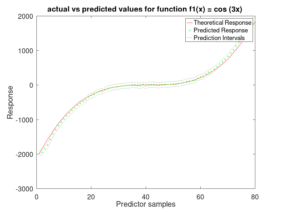
Plot the results

 figure
 [sortedY, indY] = sort (Ytrue);
 plot (sortedY, 'r-');
 xlim ([0, 80]);
 hold on
 plot (ypred(indY), 'g+')
 plot (yInt(indY,1), 'k:')
 plot (yInt(indY,2), 'k:')
 xlabel ('Predictor samples');
 ylabel ('Response');
 title ('actual vs predicted values for function f1(x) = cos (3x) ');
 legend ({'Theoretical Response', 'Predicted Response', 'Prediction Intervals'});

Use 30% Holdout partitioning for training and testing data

 C = cvpartition (80, 'HoldOut', 0.3);
 [ypred, ySDsd, yInt] = predict (a, X(test (C),:));

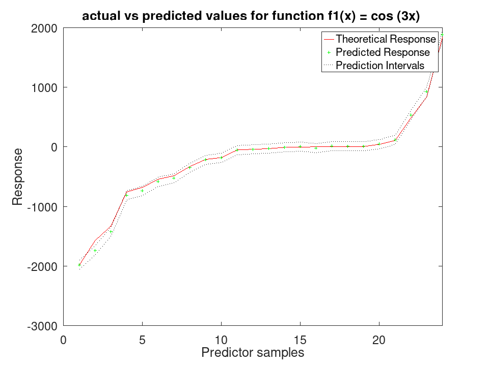
Plot the results

 figure
 [sortedY, indY] = sort (Ytrue(test (C)));
 plot (sortedY, 'r-');
 xlim ([0, sum(test(C))]);
 hold on
 plot (ypred(indY), 'g+')
 plot (yInt(indY,1),'k:')
 plot (yInt(indY,2),'k:')
 xlabel ('Predictor samples');
 ylabel ('Response');
 title ('actual vs predicted values for function f1(x) = cos (3x) ');
 legend ({'Theoretical Response', 'Predicted Response', 'Prediction Intervals'});

A numeric column vector with one entry per observation used for training, the 'Weights' normalised to sum to one, and equal when none were given. It has the class of the 'Weights' given, single or double. This property is read-only.

Train a RegressionGAM Model for synthetic values

 rng (42);
 f1 = @(x) cos (3 * x);
 f2 = @(x) x .^ 3;
 x1 = 2 * rand (50, 1) - 1;
 x2 = 2 * rand (50, 1) - 1;
 y = f1(x1) + f2(x2);
 y = y + y .* 0.2 .* rand (50,1);
 X = [x1, x2];
 a = fitrgam (X, y)

a =

  RegressionGAM

             ResponseName: 'Y'
          NumObservations: 50
            NumPredictors: 2
        ResponseTransform: 'none'
                Intercept: 0.0671178
                    Knots: []
                    Order: []
                      Tol:

Declare two different functions

 rng (42);
 f1 = @(x) cos (3 * x);
 f2 = @(x) x .^ 3;

Generate 80 samples for f1 and f2

 x = [-4*pi:0.1*pi:4*pi-0.1*pi]';
 X1 = f1(x);
 X2 = f2(x);

Create a synthetic response by adding noise

 Ytrue = X1 + X2;
 Y = Ytrue + Ytrue .* 0.2 .* rand (80,1);

Assemble predictor data

 X = [X1, X2];

Train the GAM and test on the same data A standard deviation and a prediction interval come from the spline engine, which fits one; the boosted-tree engine reports none.

 a = fitrgam (X, Y, 'FitMethod', 'splines', 'order', [5, 5]);
 [ypred, ySDsd, yInt] = predict (a, X);

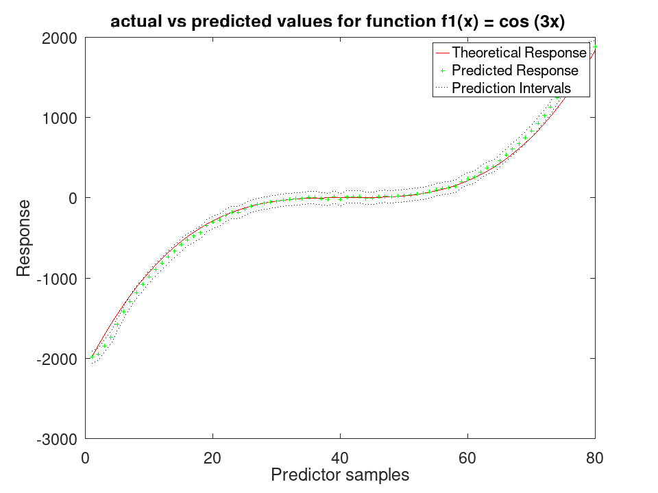
Plot the results

 figure
 [sortedY, indY] = sort (Ytrue);
 plot (sortedY, 'r-');
 xlim ([0, 80]);
 hold on
 plot (ypred(indY), 'g+')
 plot (yInt(indY,1), 'k:')
 plot (yInt(indY,2), 'k:')
 xlabel ('Predictor samples');
 ylabel ('Response');
 title ('actual vs predicted values for function f1(x) = cos (3x) ');
 legend ({'Theoretical Response', 'Predicted Response', 'Prediction Intervals'});

Use 30% Holdout partitioning for training and testing data

 C = cvpartition (80, 'HoldOut', 0.3);
 [ypred, ySDsd, yInt] = predict (a, X(test (C),:));

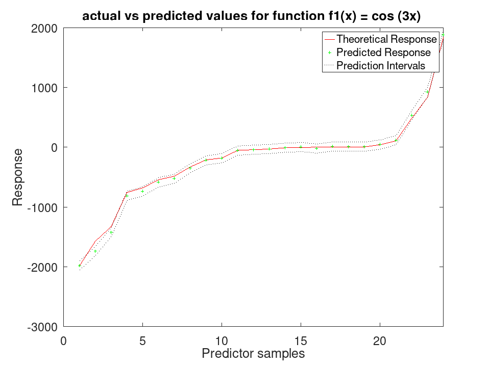
Plot the results

 figure
 [sortedY, indY] = sort (Ytrue(test (C)));
 plot (sortedY, 'r-');
 xlim ([0, sum(test(C))]);
 hold on
 plot (ypred(indY), 'g+')
 plot (yInt(indY,1),'k:')
 plot (yInt(indY,2),'k:')
 xlabel ('Predictor samples');
 ylabel ('Response');
 title ('actual vs predicted values for function f1(x) = cos (3x) ');
 legend ({'Theoretical Response', 'Predicted Response', 'Prediction Intervals'});

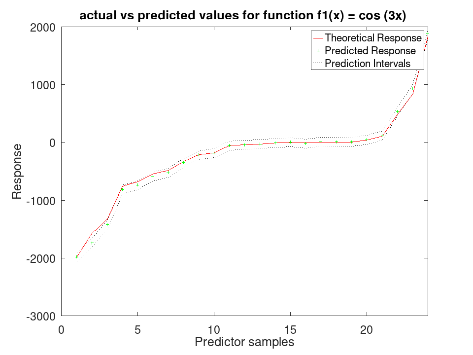
A numeric scalar, the mean of the response, which every additive term is measured against. This property is read-only.

Train a RegressionGAM Model for synthetic values

 rng (42);
 f1 = @(x) cos (3 * x);
 f2 = @(x) x .^ 3;
 x1 = 2 * rand (50, 1) - 1;
 x2 = 2 * rand (50, 1) - 1;
 y = f1(x1) + f2(x2);
 y = y + y .* 0.2 .* rand (50,1);
 X = [x1, x2];
 a = fitrgam (X, y)

a =

  RegressionGAM

             ResponseName: 'Y'
          NumObservations: 50
            NumPredictors: 2
        ResponseTransform: 'none'
                Intercept: 0.0671178
                    Knots: []
                    Order: []
                      Tol:

Declare two different functions

 rng (42);
 f1 = @(x) cos (3 * x);
 f2 = @(x) x .^ 3;

Generate 80 samples for f1 and f2

 x = [-4*pi:0.1*pi:4*pi-0.1*pi]';
 X1 = f1(x);
 X2 = f2(x);

Create a synthetic response by adding noise

 Ytrue = X1 + X2;
 Y = Ytrue + Ytrue .* 0.2 .* rand (80,1);

Assemble predictor data

 X = [X1, X2];

Train the GAM and test on the same data A standard deviation and a prediction interval come from the spline engine, which fits one; the boosted-tree engine reports none.

 a = fitrgam (X, Y, 'FitMethod', 'splines', 'order', [5, 5]);
 [ypred, ySDsd, yInt] = predict (a, X);

Plot the results

 figure
 [sortedY, indY] = sort (Ytrue);
 plot (sortedY, 'r-');
 xlim ([0, 80]);
 hold on
 plot (ypred(indY), 'g+')
 plot (yInt(indY,1), 'k:')
 plot (yInt(indY,2), 'k:')
 xlabel ('Predictor samples');
 ylabel ('Response');
 title ('actual vs predicted values for function f1(x) = cos (3x) ');
 legend ({'Theoretical Response', 'Predicted Response', 'Prediction Intervals'});

Use 30% Holdout partitioning for training and testing data

 C = cvpartition (80, 'HoldOut', 0.3);
 [ypred, ySDsd, yInt] = predict (a, X(test (C),:));

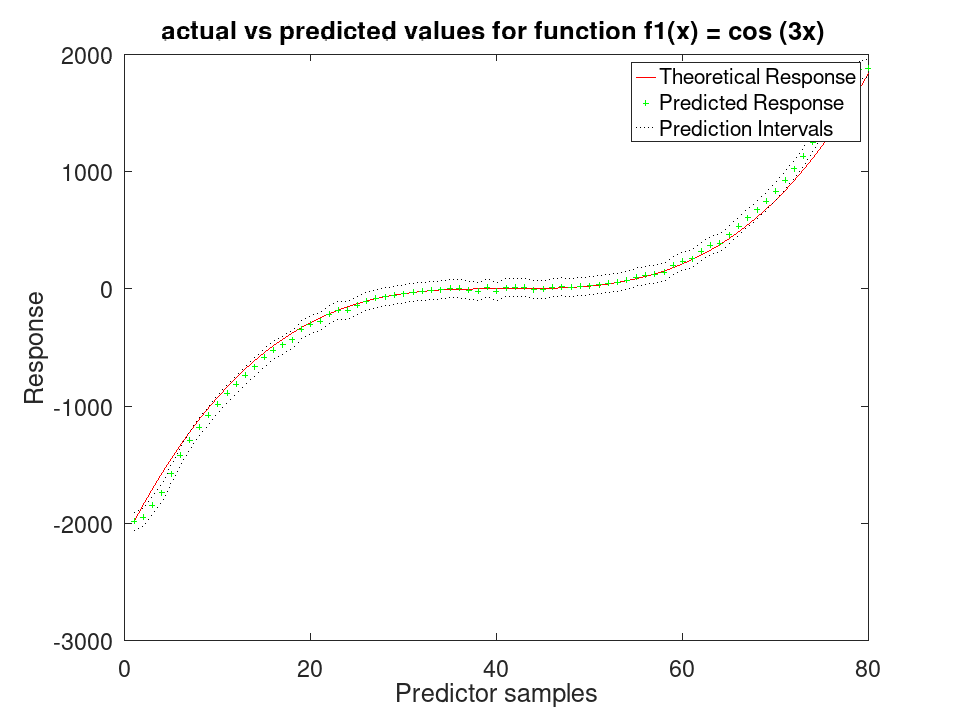
Plot the results

 figure
 [sortedY, indY] = sort (Ytrue(test (C)));
 plot (sortedY, 'r-');
 xlim ([0, sum(test(C))]);
 hold on
 plot (ypred(indY), 'g+')
 plot (yInt(indY,1),'k:')
 plot (yInt(indY,2),'k:')
 xlabel ('Predictor samples');
 ylabel ('Response');
 title ('actual vs predicted values for function f1(x) = cos (3x) ');
 legend ({'Theoretical Response', 'Predicted Response', 'Prediction Intervals'});

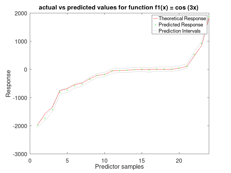
A character vector naming the response and the terms of the model, as in 'Y ~ x1 + x2 + x1:x2', or empty when the model was not given one. This property is read-only.

Train a RegressionGAM Model for synthetic values

 rng (42);
 f1 = @(x) cos (3 * x);
 f2 = @(x) x .^ 3;
 x1 = 2 * rand (50, 1) - 1;
 x2 = 2 * rand (50, 1) - 1;
 y = f1(x1) + f2(x2);
 y = y + y .* 0.2 .* rand (50,1);
 X = [x1, x2];
 a = fitrgam (X, y)

a =

  RegressionGAM

             ResponseName: 'Y'
          NumObservations: 50
            NumPredictors: 2
        ResponseTransform: 'none'
                Intercept: 0.0671178
                    Knots: []
                    Order: []
                      Tol:

Declare two different functions

 rng (42);
 f1 = @(x) cos (3 * x);
 f2 = @(x) x .^ 3;

Generate 80 samples for f1 and f2

 x = [-4*pi:0.1*pi:4*pi-0.1*pi]';
 X1 = f1(x);
 X2 = f2(x);

Create a synthetic response by adding noise

 Ytrue = X1 + X2;
 Y = Ytrue + Ytrue .* 0.2 .* rand (80,1);

Assemble predictor data

 X = [X1, X2];

Train the GAM and test on the same data A standard deviation and a prediction interval come from the spline engine, which fits one; the boosted-tree engine reports none.

 a = fitrgam (X, Y, 'FitMethod', 'splines', 'order', [5, 5]);
 [ypred, ySDsd, yInt] = predict (a, X);

Plot the results

 figure
 [sortedY, indY] = sort (Ytrue);
 plot (sortedY, 'r-');
 xlim ([0, 80]);
 hold on
 plot (ypred(indY), 'g+')
 plot (yInt(indY,1), 'k:')
 plot (yInt(indY,2), 'k:')
 xlabel ('Predictor samples');
 ylabel ('Response');
 title ('actual vs predicted values for function f1(x) = cos (3x) ');
 legend ({'Theoretical Response', 'Predicted Response', 'Prediction Intervals'});

Use 30% Holdout partitioning for training and testing data

 C = cvpartition (80, 'HoldOut', 0.3);
 [ypred, ySDsd, yInt] = predict (a, X(test (C),:));

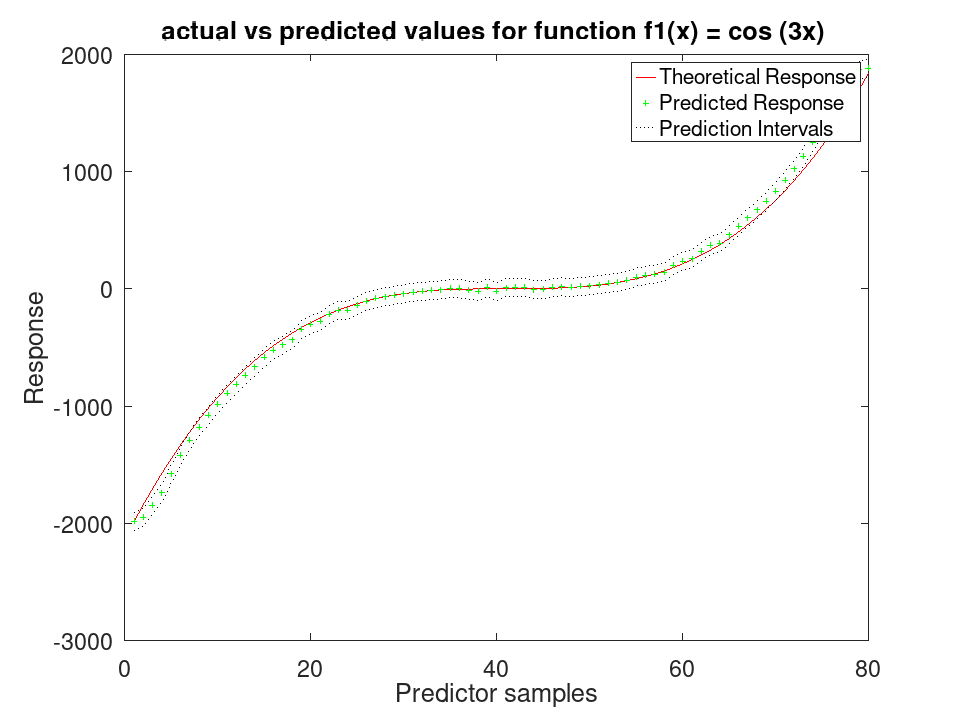
Plot the results

 figure
 [sortedY, indY] = sort (Ytrue(test (C)));
 plot (sortedY, 'r-');
 xlim ([0, sum(test(C))]);
 hold on
 plot (ypred(indY), 'g+')
 plot (yInt(indY,1),'k:')
 plot (yInt(indY,2),'k:')
 xlabel ('Predictor samples');
 ylabel ('Response');
 title ('actual vs predicted values for function f1(x) = cos (3x) ');
 legend ({'Theoretical Response', 'Predicted Response', 'Prediction Intervals'});

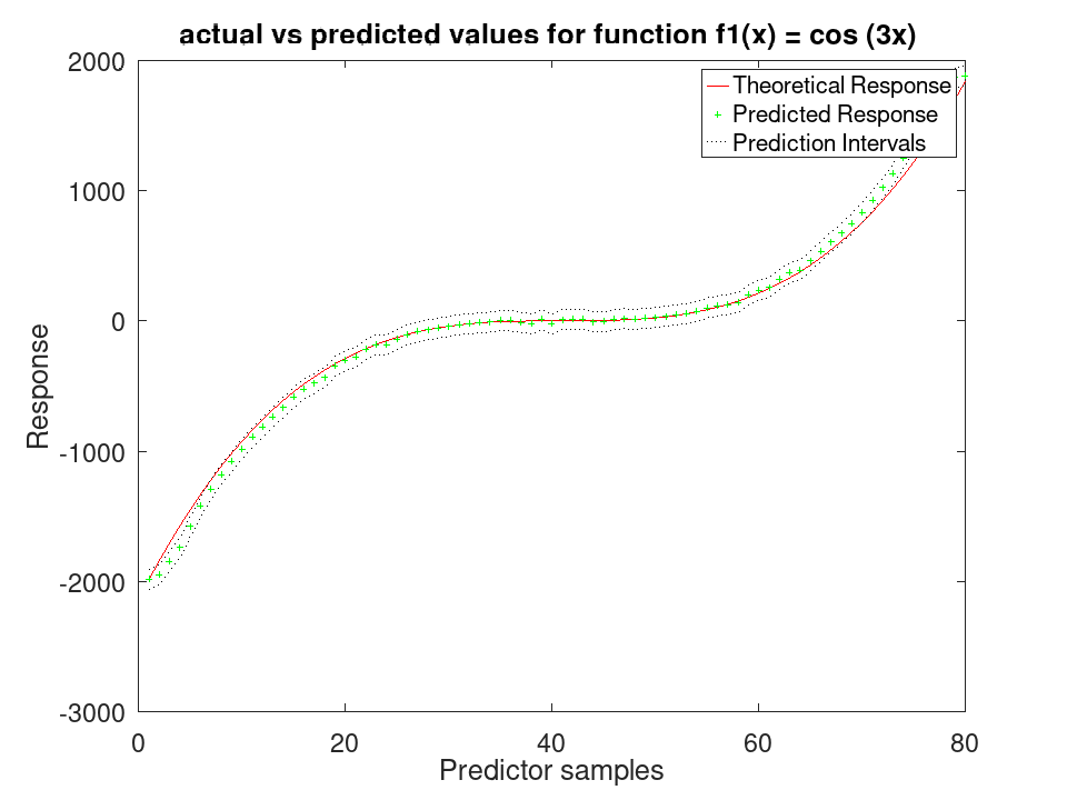
A Kx2 matrix of predictor index pairs, one row per two-way term the model carries, and zeros (0, 2) when it carries none. It reports what was fitted rather than what was asked for, so a count of terms, 'all', a logical matrix and a formula all leave the same kind of value behind. This property is read-only.

A main effect names one predictor and a higher-order term names three or more, and neither has a two-column form, so neither appears here. IntMatrix remains the complete record of every term fitted.

Train a RegressionGAM Model for synthetic values

 rng (42);
 f1 = @(x) cos (3 * x);
 f2 = @(x) x .^ 3;
 x1 = 2 * rand (50, 1) - 1;
 x2 = 2 * rand (50, 1) - 1;
 y = f1(x1) + f2(x2);
 y = y + y .* 0.2 .* rand (50,1);
 X = [x1, x2];
 a = fitrgam (X, y)

a =

  RegressionGAM

             ResponseName: 'Y'
          NumObservations: 50
            NumPredictors: 2
        ResponseTransform: 'none'
                Intercept: 0.0671178
                    Knots: []
                    Order: []
                      Tol:

Declare two different functions

 rng (42);
 f1 = @(x) cos (3 * x);
 f2 = @(x) x .^ 3;

Generate 80 samples for f1 and f2

 x = [-4*pi:0.1*pi:4*pi-0.1*pi]';
 X1 = f1(x);
 X2 = f2(x);

Create a synthetic response by adding noise

 Ytrue = X1 + X2;
 Y = Ytrue + Ytrue .* 0.2 .* rand (80,1);

Assemble predictor data

 X = [X1, X2];

Train the GAM and test on the same data A standard deviation and a prediction interval come from the spline engine, which fits one; the boosted-tree engine reports none.

 a = fitrgam (X, Y, 'FitMethod', 'splines', 'order', [5, 5]);
 [ypred, ySDsd, yInt] = predict (a, X);

Plot the results

 figure
 [sortedY, indY] = sort (Ytrue);
 plot (sortedY, 'r-');
 xlim ([0, 80]);
 hold on
 plot (ypred(indY), 'g+')
 plot (yInt(indY,1), 'k:')
 plot (yInt(indY,2), 'k:')
 xlabel ('Predictor samples');
 ylabel ('Response');
 title ('actual vs predicted values for function f1(x) = cos (3x) ');
 legend ({'Theoretical Response', 'Predicted Response', 'Prediction Intervals'});

Use 30% Holdout partitioning for training and testing data

 C = cvpartition (80, 'HoldOut', 0.3);
 [ypred, ySDsd, yInt] = predict (a, X(test (C),:));

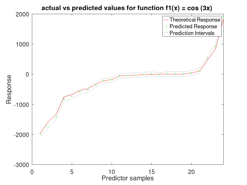
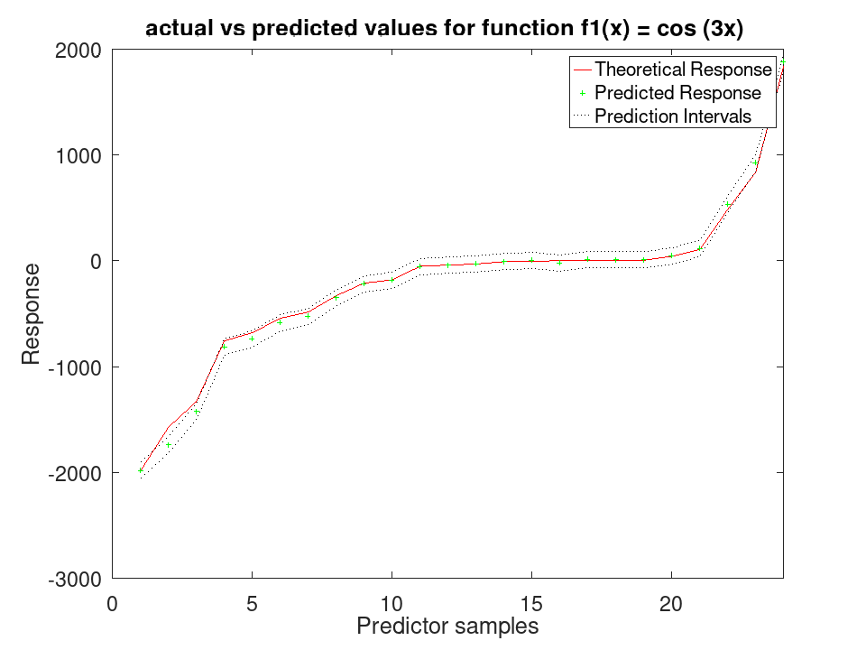
Plot the results

 figure
 [sortedY, indY] = sort (Ytrue(test (C)));
 plot (sortedY, 'r-');
 xlim ([0, sum(test(C))]);
 hold on
 plot (ypred(indY), 'g+')
 plot (yInt(indY,1),'k:')
 plot (yInt(indY,2),'k:')
 xlabel ('Predictor samples');
 ylabel ('Response');
 title ('actual vs predicted values for function f1(x) = cos (3x) ');
 legend ({'Theoretical Response', 'Predicted Response', 'Prediction Intervals'});

A numeric vector with one entry per predictor, the number of breaks the spline of that predictor is fitted over. This property is read-only.

Train a RegressionGAM Model for synthetic values

 rng (42);
 f1 = @(x) cos (3 * x);
 f2 = @(x) x .^ 3;
 x1 = 2 * rand (50, 1) - 1;
 x2 = 2 * rand (50, 1) - 1;
 y = f1(x1) + f2(x2);
 y = y + y .* 0.2 .* rand (50,1);
 X = [x1, x2];
 a = fitrgam (X, y)

a =

  RegressionGAM

             ResponseName: 'Y'
          NumObservations: 50
            NumPredictors: 2
        ResponseTransform: 'none'
                Intercept: 0.0671178
                    Knots: []
                    Order: []
                      Tol:

Declare two different functions

 rng (42);
 f1 = @(x) cos (3 * x);
 f2 = @(x) x .^ 3;

Generate 80 samples for f1 and f2

 x = [-4*pi:0.1*pi:4*pi-0.1*pi]';
 X1 = f1(x);
 X2 = f2(x);

Create a synthetic response by adding noise

 Ytrue = X1 + X2;
 Y = Ytrue + Ytrue .* 0.2 .* rand (80,1);

Assemble predictor data

 X = [X1, X2];

Train the GAM and test on the same data A standard deviation and a prediction interval come from the spline engine, which fits one; the boosted-tree engine reports none.

 a = fitrgam (X, Y, 'FitMethod', 'splines', 'order', [5, 5]);
 [ypred, ySDsd, yInt] = predict (a, X);

Plot the results

 figure
 [sortedY, indY] = sort (Ytrue);
 plot (sortedY, 'r-');
 xlim ([0, 80]);
 hold on
 plot (ypred(indY), 'g+')
 plot (yInt(indY,1), 'k:')
 plot (yInt(indY,2), 'k:')
 xlabel ('Predictor samples');
 ylabel ('Response');
 title ('actual vs predicted values for function f1(x) = cos (3x) ');
 legend ({'Theoretical Response', 'Predicted Response', 'Prediction Intervals'});

Use 30% Holdout partitioning for training and testing data

 C = cvpartition (80, 'HoldOut', 0.3);
 [ypred, ySDsd, yInt] = predict (a, X(test (C),:));

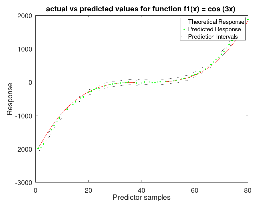
Plot the results

 figure
 [sortedY, indY] = sort (Ytrue(test (C)));
 plot (sortedY, 'r-');
 xlim ([0, sum(test(C))]);
 hold on
 plot (ypred(indY), 'g+')
 plot (yInt(indY,1),'k:')
 plot (yInt(indY,2),'k:')
 xlabel ('Predictor samples');
 ylabel ('Response');
 title ('actual vs predicted values for function f1(x) = cos (3x) ');
 legend ({'Theoretical Response', 'Predicted Response', 'Prediction Intervals'});

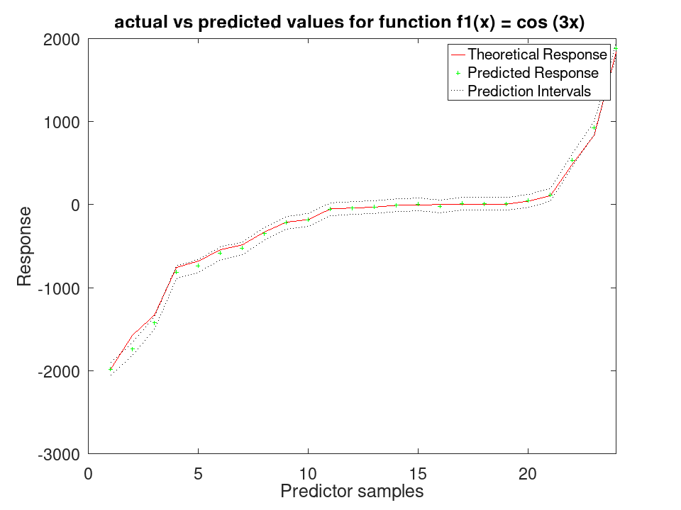
A numeric vector with one entry per predictor, the polynomial order of the spline of that predictor. This property is read-only.

Train a RegressionGAM Model for synthetic values

 rng (42);
 f1 = @(x) cos (3 * x);
 f2 = @(x) x .^ 3;
 x1 = 2 * rand (50, 1) - 1;
 x2 = 2 * rand (50, 1) - 1;
 y = f1(x1) + f2(x2);
 y = y + y .* 0.2 .* rand (50,1);
 X = [x1, x2];
 a = fitrgam (X, y)

a =

  RegressionGAM

             ResponseName: 'Y'
          NumObservations: 50
            NumPredictors: 2
        ResponseTransform: 'none'
                Intercept: 0.0671178
                    Knots: []
                    Order: []
                      Tol:

Declare two different functions

 rng (42);
 f1 = @(x) cos (3 * x);
 f2 = @(x) x .^ 3;

Generate 80 samples for f1 and f2

 x = [-4*pi:0.1*pi:4*pi-0.1*pi]';
 X1 = f1(x);
 X2 = f2(x);

Create a synthetic response by adding noise

 Ytrue = X1 + X2;
 Y = Ytrue + Ytrue .* 0.2 .* rand (80,1);

Assemble predictor data

 X = [X1, X2];

Train the GAM and test on the same data A standard deviation and a prediction interval come from the spline engine, which fits one; the boosted-tree engine reports none.

 a = fitrgam (X, Y, 'FitMethod', 'splines', 'order', [5, 5]);
 [ypred, ySDsd, yInt] = predict (a, X);

Plot the results

 figure
 [sortedY, indY] = sort (Ytrue);
 plot (sortedY, 'r-');
 xlim ([0, 80]);
 hold on
 plot (ypred(indY), 'g+')
 plot (yInt(indY,1), 'k:')
 plot (yInt(indY,2), 'k:')
 xlabel ('Predictor samples');
 ylabel ('Response');
 title ('actual vs predicted values for function f1(x) = cos (3x) ');
 legend ({'Theoretical Response', 'Predicted Response', 'Prediction Intervals'});

Use 30% Holdout partitioning for training and testing data

 C = cvpartition (80, 'HoldOut', 0.3);
 [ypred, ySDsd, yInt] = predict (a, X(test (C),:));

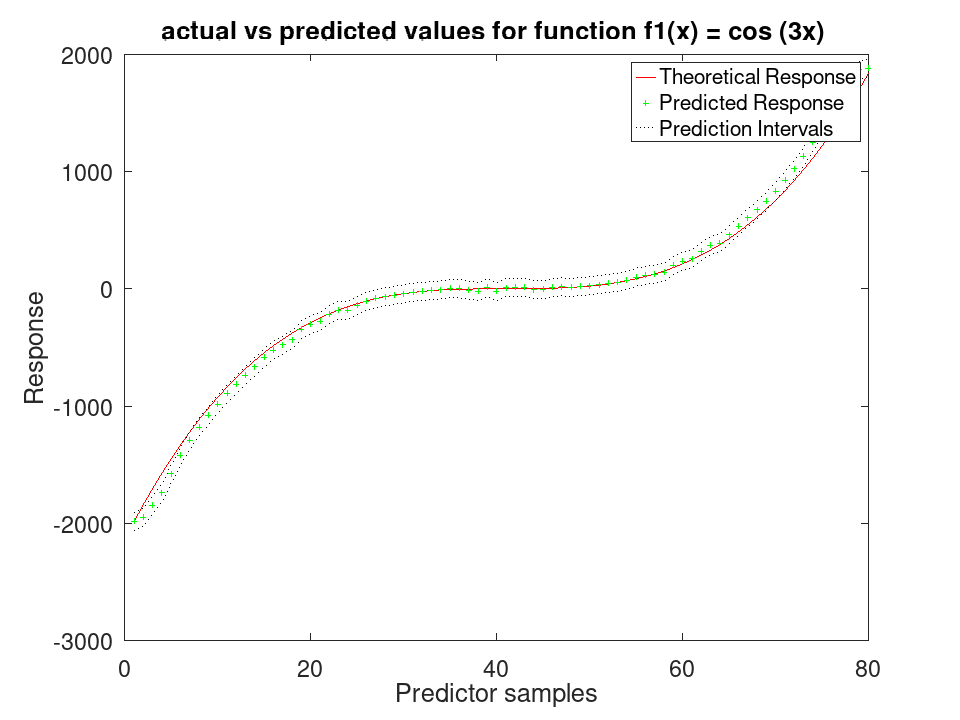
Plot the results

 figure
 [sortedY, indY] = sort (Ytrue(test (C)));
 plot (sortedY, 'r-');
 xlim ([0, sum(test(C))]);
 hold on
 plot (ypred(indY), 'g+')
 plot (yInt(indY,1),'k:')
 plot (yInt(indY,2),'k:')
 xlabel ('Predictor samples');
 ylabel ('Response');
 title ('actual vs predicted values for function f1(x) = cos (3x) ');
 legend ({'Theoretical Response', 'Predicted Response', 'Prediction Intervals'});

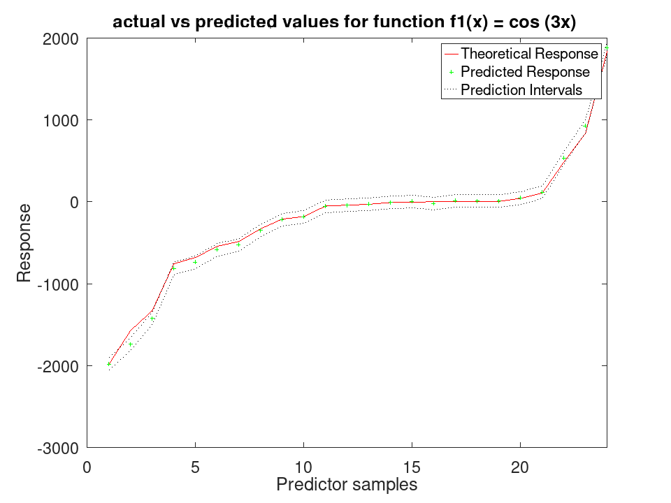
A numeric vector with one entry per predictor, the sum of its number of knots and its order. This property is read-only.

Train a RegressionGAM Model for synthetic values

 rng (42);
 f1 = @(x) cos (3 * x);
 f2 = @(x) x .^ 3;
 x1 = 2 * rand (50, 1) - 1;
 x2 = 2 * rand (50, 1) - 1;
 y = f1(x1) + f2(x2);
 y = y + y .* 0.2 .* rand (50,1);
 X = [x1, x2];
 a = fitrgam (X, y)

a =

  RegressionGAM

             ResponseName: 'Y'
          NumObservations: 50
            NumPredictors: 2
        ResponseTransform: 'none'
                Intercept: 0.0671178
                    Knots: []
                    Order: []
                      Tol:

Declare two different functions

 rng (42);
 f1 = @(x) cos (3 * x);
 f2 = @(x) x .^ 3;

Generate 80 samples for f1 and f2

 x = [-4*pi:0.1*pi:4*pi-0.1*pi]';
 X1 = f1(x);
 X2 = f2(x);

Create a synthetic response by adding noise

 Ytrue = X1 + X2;
 Y = Ytrue + Ytrue .* 0.2 .* rand (80,1);

Assemble predictor data

 X = [X1, X2];

Train the GAM and test on the same data A standard deviation and a prediction interval come from the spline engine, which fits one; the boosted-tree engine reports none.

 a = fitrgam (X, Y, 'FitMethod', 'splines', 'order', [5, 5]);
 [ypred, ySDsd, yInt] = predict (a, X);

Plot the results

 figure
 [sortedY, indY] = sort (Ytrue);
 plot (sortedY, 'r-');
 xlim ([0, 80]);
 hold on
 plot (ypred(indY), 'g+')
 plot (yInt(indY,1), 'k:')
 plot (yInt(indY,2), 'k:')
 xlabel ('Predictor samples');
 ylabel ('Response');
 title ('actual vs predicted values for function f1(x) = cos (3x) ');
 legend ({'Theoretical Response', 'Predicted Response', 'Prediction Intervals'});

Use 30% Holdout partitioning for training and testing data

 C = cvpartition (80, 'HoldOut', 0.3);
 [ypred, ySDsd, yInt] = predict (a, X(test (C),:));

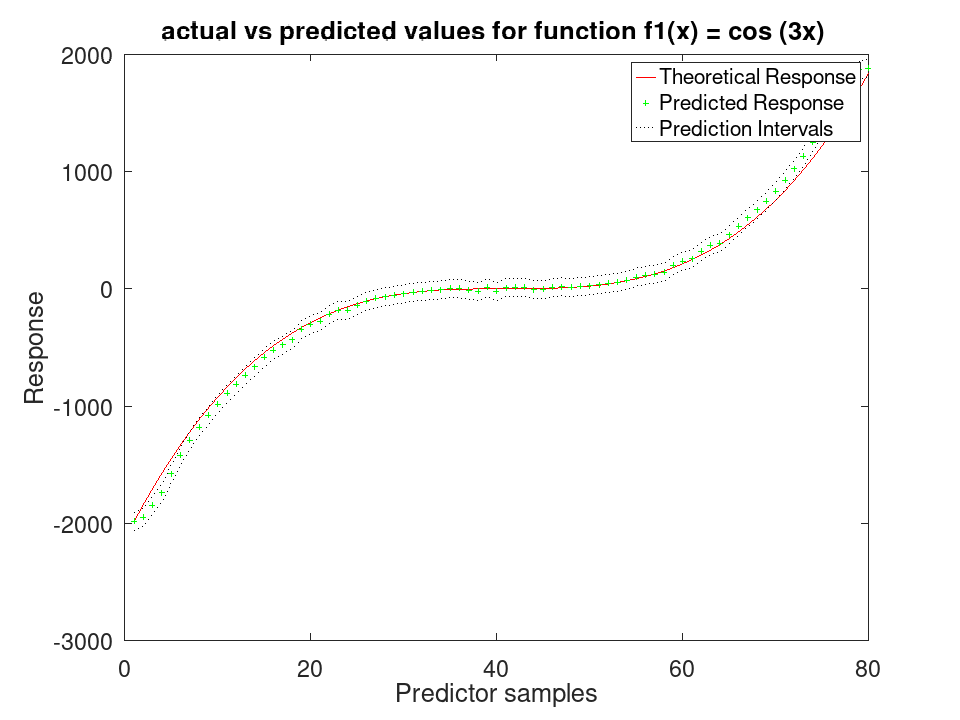
Plot the results

 figure
 [sortedY, indY] = sort (Ytrue(test (C)));
 plot (sortedY, 'r-');
 xlim ([0, sum(test(C))]);
 hold on
 plot (ypred(indY), 'g+')
 plot (yInt(indY,1),'k:')
 plot (yInt(indY,2),'k:')
 xlabel ('Predictor samples');
 ylabel ('Response');
 title ('actual vs predicted values for function f1(x) = cos (3x) ');
 legend ({'Theoretical Response', 'Predicted Response', 'Prediction Intervals'});

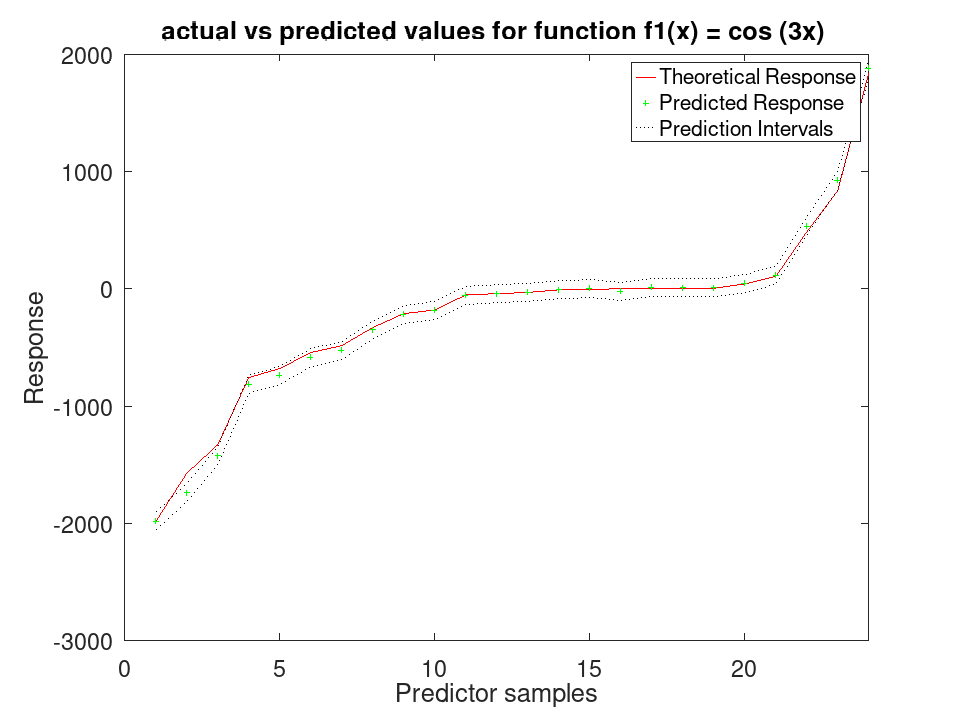
A positive scalar, the largest change in the residual sum of squares of a backfitting cycle that counts as converged. This property is read-only.

Train a RegressionGAM Model for synthetic values

 rng (42);
 f1 = @(x) cos (3 * x);
 f2 = @(x) x .^ 3;
 x1 = 2 * rand (50, 1) - 1;
 x2 = 2 * rand (50, 1) - 1;
 y = f1(x1) + f2(x2);
 y = y + y .* 0.2 .* rand (50,1);
 X = [x1, x2];
 a = fitrgam (X, y)

a =

  RegressionGAM

             ResponseName: 'Y'
          NumObservations: 50
            NumPredictors: 2
        ResponseTransform: 'none'
                Intercept: 0.0671178
                    Knots: []
                    Order: []
                      Tol:

Declare two different functions

 rng (42);
 f1 = @(x) cos (3 * x);
 f2 = @(x) x .^ 3;

Generate 80 samples for f1 and f2

 x = [-4*pi:0.1*pi:4*pi-0.1*pi]';
 X1 = f1(x);
 X2 = f2(x);

Create a synthetic response by adding noise

 Ytrue = X1 + X2;
 Y = Ytrue + Ytrue .* 0.2 .* rand (80,1);

Assemble predictor data

 X = [X1, X2];

Train the GAM and test on the same data A standard deviation and a prediction interval come from the spline engine, which fits one; the boosted-tree engine reports none.

 a = fitrgam (X, Y, 'FitMethod', 'splines', 'order', [5, 5]);
 [ypred, ySDsd, yInt] = predict (a, X);

Plot the results

 figure
 [sortedY, indY] = sort (Ytrue);
 plot (sortedY, 'r-');
 xlim ([0, 80]);
 hold on
 plot (ypred(indY), 'g+')
 plot (yInt(indY,1), 'k:')
 plot (yInt(indY,2), 'k:')
 xlabel ('Predictor samples');
 ylabel ('Response');
 title ('actual vs predicted values for function f1(x) = cos (3x) ');
 legend ({'Theoretical Response', 'Predicted Response', 'Prediction Intervals'});

Use 30% Holdout partitioning for training and testing data

 C = cvpartition (80, 'HoldOut', 0.3);
 [ypred, ySDsd, yInt] = predict (a, X(test (C),:));

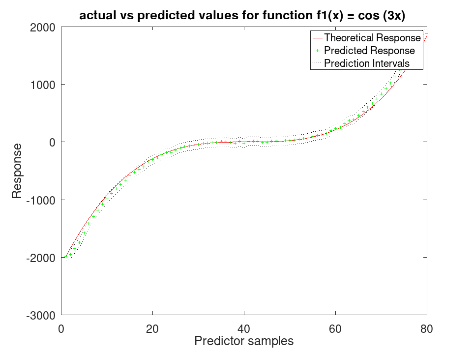
Plot the results

 figure
 [sortedY, indY] = sort (Ytrue(test (C)));
 plot (sortedY, 'r-');
 xlim ([0, sum(test(C))]);
 hold on
 plot (ypred(indY), 'g+')
 plot (yInt(indY,1),'k:')
 plot (yInt(indY,2),'k:')
 xlabel ('Predictor samples');
 ylabel ('Response');
 title ('actual vs predicted values for function f1(x) = cos (3x) ');
 legend ({'Theoretical Response', 'Predicted Response', 'Prediction Intervals'});

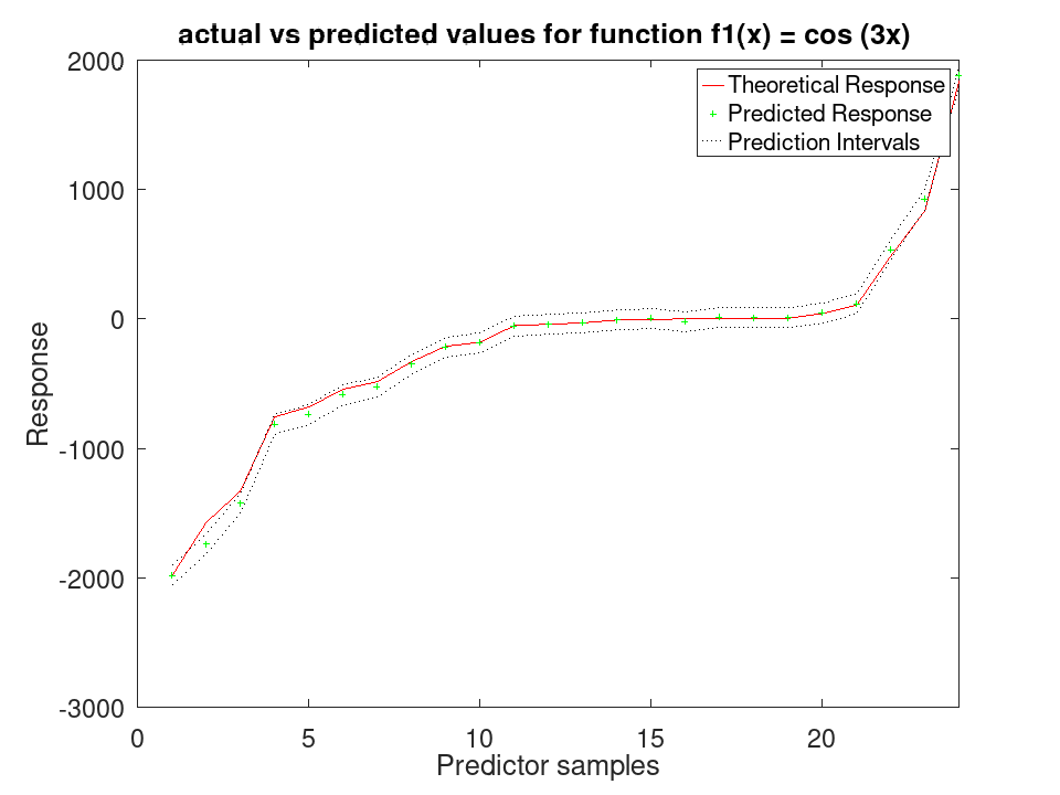
A boolean flag, always false, as this class estimates the standard deviation of a prediction from the residuals of the fit rather than fitting a model for it. This property is read-only.

Train a RegressionGAM Model for synthetic values

 rng (42);
 f1 = @(x) cos (3 * x);
 f2 = @(x) x .^ 3;
 x1 = 2 * rand (50, 1) - 1;
 x2 = 2 * rand (50, 1) - 1;
 y = f1(x1) + f2(x2);
 y = y + y .* 0.2 .* rand (50,1);
 X = [x1, x2];
 a = fitrgam (X, y)

a =

  RegressionGAM

             ResponseName: 'Y'
          NumObservations: 50
            NumPredictors: 2
        ResponseTransform: 'none'
                Intercept: 0.0671178
                    Knots: []
                    Order: []
                      Tol:

Declare two different functions

 rng (42);
 f1 = @(x) cos (3 * x);
 f2 = @(x) x .^ 3;

Generate 80 samples for f1 and f2

 x = [-4*pi:0.1*pi:4*pi-0.1*pi]';
 X1 = f1(x);
 X2 = f2(x);

Create a synthetic response by adding noise

 Ytrue = X1 + X2;
 Y = Ytrue + Ytrue .* 0.2 .* rand (80,1);

Assemble predictor data

 X = [X1, X2];

Train the GAM and test on the same data A standard deviation and a prediction interval come from the spline engine, which fits one; the boosted-tree engine reports none.

 a = fitrgam (X, Y, 'FitMethod', 'splines', 'order', [5, 5]);
 [ypred, ySDsd, yInt] = predict (a, X);

Plot the results

 figure
 [sortedY, indY] = sort (Ytrue);
 plot (sortedY, 'r-');
 xlim ([0, 80]);
 hold on
 plot (ypred(indY), 'g+')
 plot (yInt(indY,1), 'k:')
 plot (yInt(indY,2), 'k:')
 xlabel ('Predictor samples');
 ylabel ('Response');
 title ('actual vs predicted values for function f1(x) = cos (3x) ');
 legend ({'Theoretical Response', 'Predicted Response', 'Prediction Intervals'});

Use 30% Holdout partitioning for training and testing data

 C = cvpartition (80, 'HoldOut', 0.3);
 [ypred, ySDsd, yInt] = predict (a, X(test (C),:));

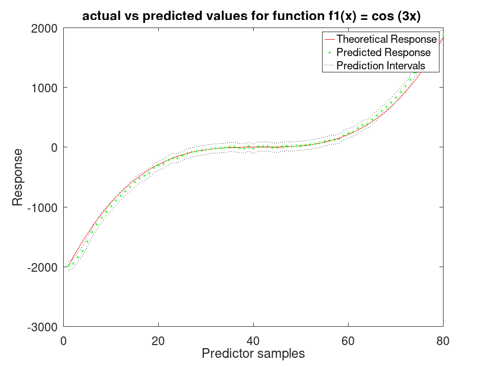
Plot the results

 figure
 [sortedY, indY] = sort (Ytrue(test (C)));
 plot (sortedY, 'r-');
 xlim ([0, sum(test(C))]);
 hold on
 plot (ypred(indY), 'g+')
 plot (yInt(indY,1),'k:')
 plot (yInt(indY,2),'k:')
 xlabel ('Predictor samples');
 ylabel ('Response');
 title ('actual vs predicted values for function f1(x) = cos (3x) ');
 legend ({'Theoretical Response', 'Predicted Response', 'Prediction Intervals'});

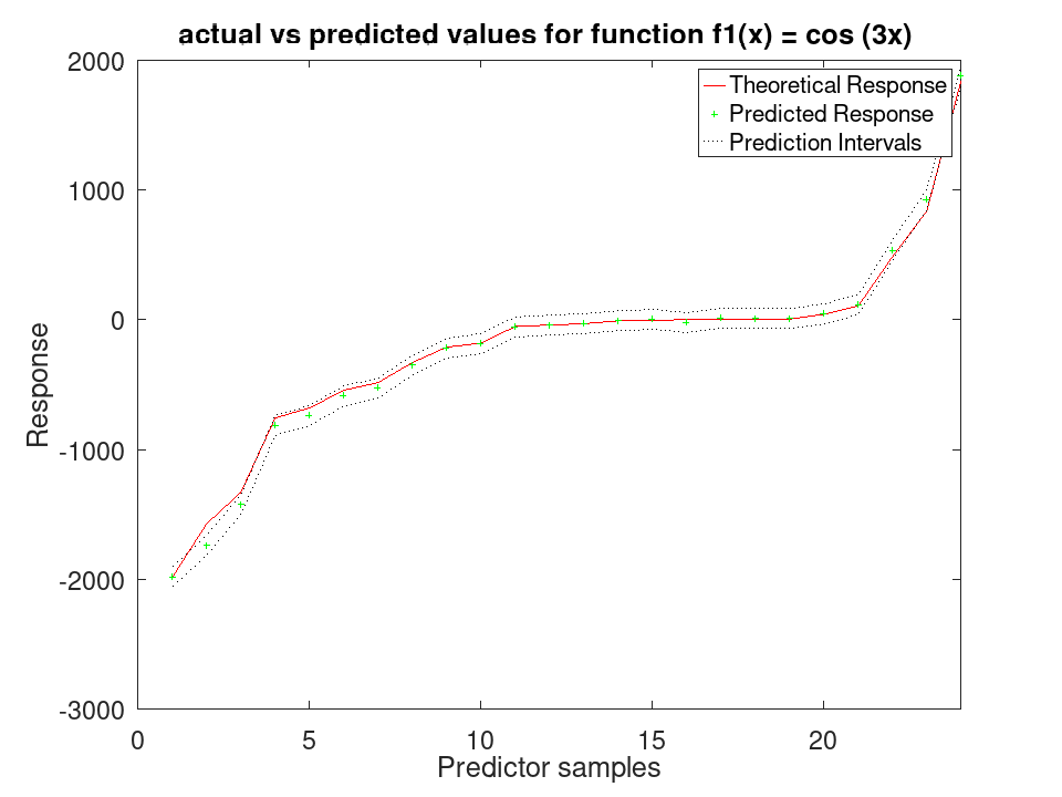
A structure holding the intercept, the piecewise polynomial of each predictor, the number of backfitting cycles, the residuals and the residual sum of squares of the model fitted without interaction terms. This property is read-only.

Train a RegressionGAM Model for synthetic values

 rng (42);
 f1 = @(x) cos (3 * x);
 f2 = @(x) x .^ 3;
 x1 = 2 * rand (50, 1) - 1;
 x2 = 2 * rand (50, 1) - 1;
 y = f1(x1) + f2(x2);
 y = y + y .* 0.2 .* rand (50,1);
 X = [x1, x2];
 a = fitrgam (X, y)

a =

  RegressionGAM

             ResponseName: 'Y'
          NumObservations: 50
            NumPredictors: 2
        ResponseTransform: 'none'
                Intercept: 0.0671178
                    Knots: []
                    Order: []
                      Tol:

Declare two different functions

 rng (42);
 f1 = @(x) cos (3 * x);
 f2 = @(x) x .^ 3;

Generate 80 samples for f1 and f2

 x = [-4*pi:0.1*pi:4*pi-0.1*pi]';
 X1 = f1(x);
 X2 = f2(x);

Create a synthetic response by adding noise

 Ytrue = X1 + X2;
 Y = Ytrue + Ytrue .* 0.2 .* rand (80,1);

Assemble predictor data

 X = [X1, X2];

Train the GAM and test on the same data A standard deviation and a prediction interval come from the spline engine, which fits one; the boosted-tree engine reports none.

 a = fitrgam (X, Y, 'FitMethod', 'splines', 'order', [5, 5]);
 [ypred, ySDsd, yInt] = predict (a, X);

Plot the results

 figure
 [sortedY, indY] = sort (Ytrue);
 plot (sortedY, 'r-');
 xlim ([0, 80]);
 hold on
 plot (ypred(indY), 'g+')
 plot (yInt(indY,1), 'k:')
 plot (yInt(indY,2), 'k:')
 xlabel ('Predictor samples');
 ylabel ('Response');
 title ('actual vs predicted values for function f1(x) = cos (3x) ');
 legend ({'Theoretical Response', 'Predicted Response', 'Prediction Intervals'});

Use 30% Holdout partitioning for training and testing data

 C = cvpartition (80, 'HoldOut', 0.3);
 [ypred, ySDsd, yInt] = predict (a, X(test (C),:));

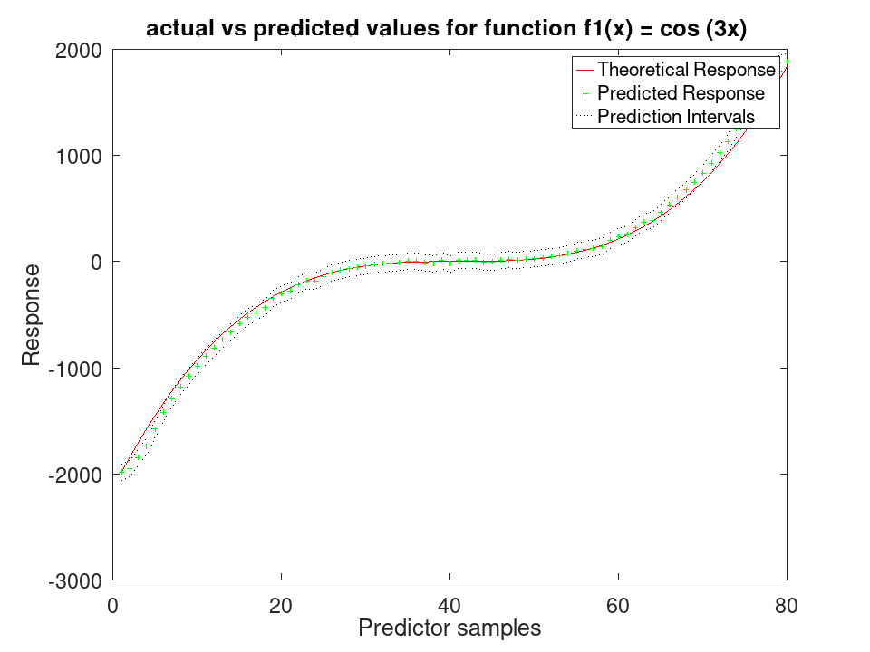
Plot the results

 figure
 [sortedY, indY] = sort (Ytrue(test (C)));
 plot (sortedY, 'r-');
 xlim ([0, sum(test(C))]);
 hold on
 plot (ypred(indY), 'g+')
 plot (yInt(indY,1),'k:')
 plot (yInt(indY,2),'k:')
 xlabel ('Predictor samples');
 ylabel ('Response');
 title ('actual vs predicted values for function f1(x) = cos (3x) ');
 legend ({'Theoretical Response', 'Predicted Response', 'Prediction Intervals'});

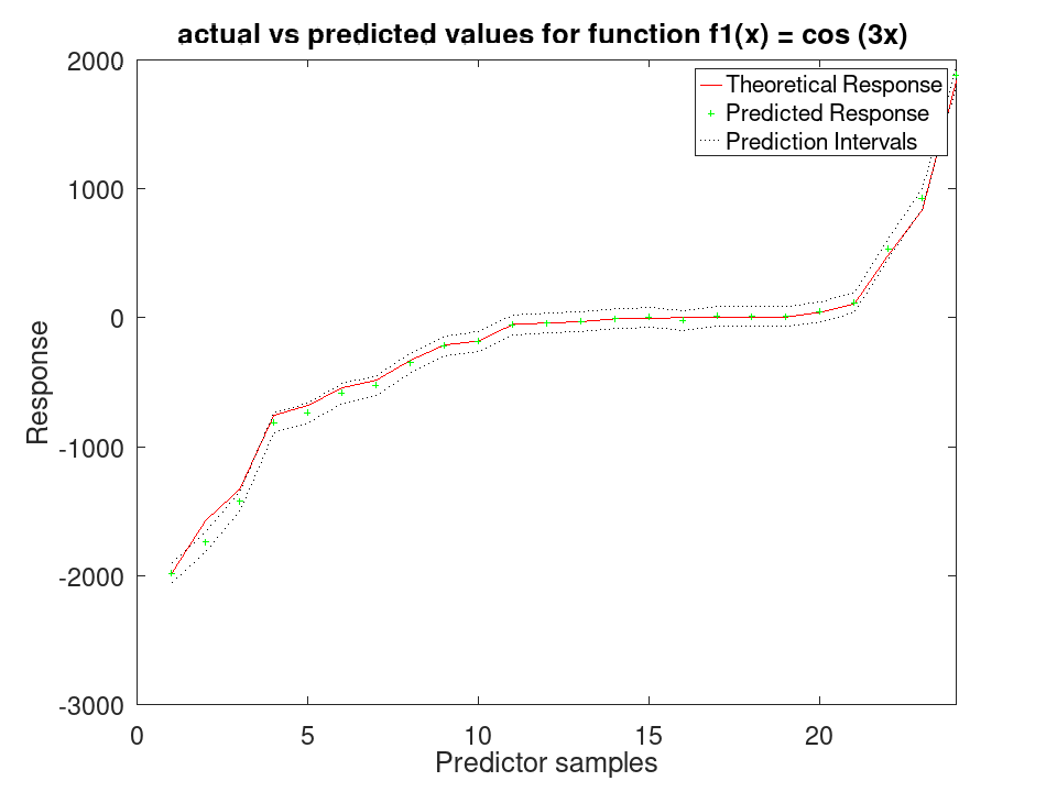
A structure of the same fields as BaseModel, for the model fitted with the interaction terms, and empty when none was asked for. This property is read-only.

Train a RegressionGAM Model for synthetic values

 rng (42);
 f1 = @(x) cos (3 * x);
 f2 = @(x) x .^ 3;
 x1 = 2 * rand (50, 1) - 1;
 x2 = 2 * rand (50, 1) - 1;
 y = f1(x1) + f2(x2);
 y = y + y .* 0.2 .* rand (50,1);
 X = [x1, x2];
 a = fitrgam (X, y)

a =

  RegressionGAM

             ResponseName: 'Y'
          NumObservations: 50
            NumPredictors: 2
        ResponseTransform: 'none'
                Intercept: 0.0671178
                    Knots: []
                    Order: []
                      Tol:

Declare two different functions

 rng (42);
 f1 = @(x) cos (3 * x);
 f2 = @(x) x .^ 3;

Generate 80 samples for f1 and f2

 x = [-4*pi:0.1*pi:4*pi-0.1*pi]';
 X1 = f1(x);
 X2 = f2(x);

Create a synthetic response by adding noise

 Ytrue = X1 + X2;
 Y = Ytrue + Ytrue .* 0.2 .* rand (80,1);

Assemble predictor data

 X = [X1, X2];

Train the GAM and test on the same data A standard deviation and a prediction interval come from the spline engine, which fits one; the boosted-tree engine reports none.

 a = fitrgam (X, Y, 'FitMethod', 'splines', 'order', [5, 5]);
 [ypred, ySDsd, yInt] = predict (a, X);

Plot the results

 figure
 [sortedY, indY] = sort (Ytrue);
 plot (sortedY, 'r-');
 xlim ([0, 80]);
 hold on
 plot (ypred(indY), 'g+')
 plot (yInt(indY,1), 'k:')
 plot (yInt(indY,2), 'k:')
 xlabel ('Predictor samples');
 ylabel ('Response');
 title ('actual vs predicted values for function f1(x) = cos (3x) ');
 legend ({'Theoretical Response', 'Predicted Response', 'Prediction Intervals'});

Use 30% Holdout partitioning for training and testing data

 C = cvpartition (80, 'HoldOut', 0.3);
 [ypred, ySDsd, yInt] = predict (a, X(test (C),:));

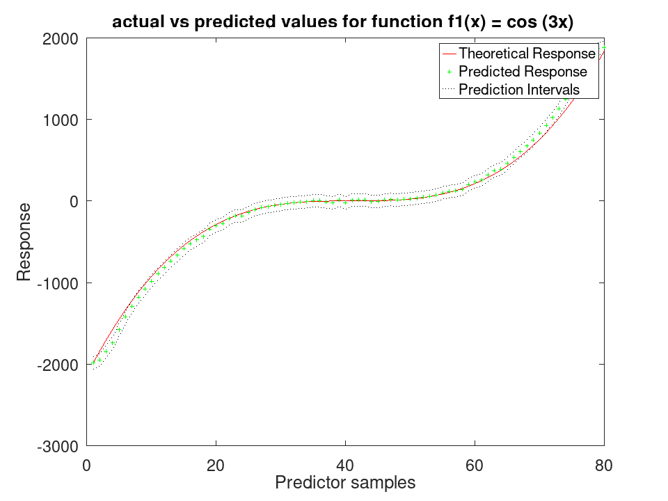
Plot the results

 figure
 [sortedY, indY] = sort (Ytrue(test (C)));
 plot (sortedY, 'r-');
 xlim ([0, sum(test(C))]);
 hold on
 plot (ypred(indY), 'g+')
 plot (yInt(indY,1),'k:')
 plot (yInt(indY,2),'k:')
 xlabel ('Predictor samples');
 ylabel ('Response');
 title ('actual vs predicted values for function f1(x) = cos (3x) ');
 legend ({'Theoretical Response', 'Predicted Response', 'Prediction Intervals'});

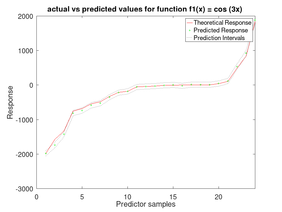
A logical matrix with one row per term and one column per predictor, true wherever the term multiplies that predictor. A row naming one predictor is a main effect, two an interaction, and three or more a higher-order term. This property is read-only.

It is the complete record, where Interactions reports only the two-way terms, in the form MATLAB reports them. It is also the form the 'Interactions' option takes back, so passing it to the constructor rebuilds a model over the same terms.

Train a RegressionGAM Model for synthetic values

 rng (42);
 f1 = @(x) cos (3 * x);
 f2 = @(x) x .^ 3;
 x1 = 2 * rand (50, 1) - 1;
 x2 = 2 * rand (50, 1) - 1;
 y = f1(x1) + f2(x2);
 y = y + y .* 0.2 .* rand (50,1);
 X = [x1, x2];
 a = fitrgam (X, y)

a =

  RegressionGAM

             ResponseName: 'Y'
          NumObservations: 50
            NumPredictors: 2
        ResponseTransform: 'none'
                Intercept: 0.0671178
                    Knots: []
                    Order: []
                      Tol:

Declare two different functions

 rng (42);
 f1 = @(x) cos (3 * x);
 f2 = @(x) x .^ 3;

Generate 80 samples for f1 and f2

 x = [-4*pi:0.1*pi:4*pi-0.1*pi]';
 X1 = f1(x);
 X2 = f2(x);

Create a synthetic response by adding noise

 Ytrue = X1 + X2;
 Y = Ytrue + Ytrue .* 0.2 .* rand (80,1);

Assemble predictor data

 X = [X1, X2];

Train the GAM and test on the same data A standard deviation and a prediction interval come from the spline engine, which fits one; the boosted-tree engine reports none.

 a = fitrgam (X, Y, 'FitMethod', 'splines', 'order', [5, 5]);
 [ypred, ySDsd, yInt] = predict (a, X);

Plot the results

 figure
 [sortedY, indY] = sort (Ytrue);
 plot (sortedY, 'r-');
 xlim ([0, 80]);
 hold on
 plot (ypred(indY), 'g+')
 plot (yInt(indY,1), 'k:')
 plot (yInt(indY,2), 'k:')
 xlabel ('Predictor samples');
 ylabel ('Response');
 title ('actual vs predicted values for function f1(x) = cos (3x) ');
 legend ({'Theoretical Response', 'Predicted Response', 'Prediction Intervals'});

Use 30% Holdout partitioning for training and testing data

 C = cvpartition (80, 'HoldOut', 0.3);
 [ypred, ySDsd, yInt] = predict (a, X(test (C),:));

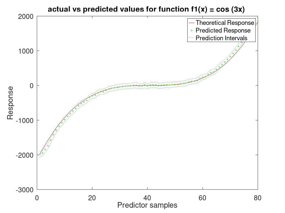
Plot the results

 figure
 [sortedY, indY] = sort (Ytrue(test (C)));
 plot (sortedY, 'r-');
 xlim ([0, sum(test(C))]);
 hold on
 plot (ypred(indY), 'g+')
 plot (yInt(indY,1),'k:')
 plot (yInt(indY,2),'k:')
 xlabel ('Predictor samples');
 ylabel ('Response');
 title ('actual vs predicted values for function f1(x) = cos (3x) ');
 legend ({'Theoretical Response', 'Predicted Response', 'Prediction Intervals'});

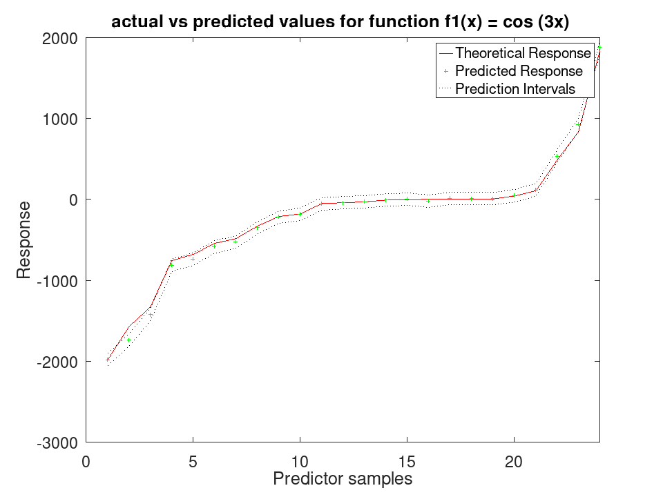
A cell array with one entry per predictor, holding that predictor’s bin edges where the model discretized it before fitting. It is empty here and stays empty: this generalized additive model is built from splines, which take the predictors as they are, where MATLAB’s is built from boosted trees and bins them. That difference is described in the class documentation.

This property is read-only.

Train a RegressionGAM Model for synthetic values

 rng (42);
 f1 = @(x) cos (3 * x);
 f2 = @(x) x .^ 3;
 x1 = 2 * rand (50, 1) - 1;
 x2 = 2 * rand (50, 1) - 1;
 y = f1(x1) + f2(x2);
 y = y + y .* 0.2 .* rand (50,1);
 X = [x1, x2];
 a = fitrgam (X, y)

a =

  RegressionGAM

             ResponseName: 'Y'
          NumObservations: 50
            NumPredictors: 2
        ResponseTransform: 'none'
                Intercept: 0.0671178
                    Knots: []
                    Order: []
                      Tol:

Declare two different functions

 rng (42);
 f1 = @(x) cos (3 * x);
 f2 = @(x) x .^ 3;

Generate 80 samples for f1 and f2

 x = [-4*pi:0.1*pi:4*pi-0.1*pi]';
 X1 = f1(x);
 X2 = f2(x);

Create a synthetic response by adding noise

 Ytrue = X1 + X2;
 Y = Ytrue + Ytrue .* 0.2 .* rand (80,1);

Assemble predictor data

 X = [X1, X2];

Train the GAM and test on the same data A standard deviation and a prediction interval come from the spline engine, which fits one; the boosted-tree engine reports none.

 a = fitrgam (X, Y, 'FitMethod', 'splines', 'order', [5, 5]);
 [ypred, ySDsd, yInt] = predict (a, X);

Plot the results

 figure
 [sortedY, indY] = sort (Ytrue);
 plot (sortedY, 'r-');
 xlim ([0, 80]);
 hold on
 plot (ypred(indY), 'g+')
 plot (yInt(indY,1), 'k:')
 plot (yInt(indY,2), 'k:')
 xlabel ('Predictor samples');
 ylabel ('Response');
 title ('actual vs predicted values for function f1(x) = cos (3x) ');
 legend ({'Theoretical Response', 'Predicted Response', 'Prediction Intervals'});

Use 30% Holdout partitioning for training and testing data

 C = cvpartition (80, 'HoldOut', 0.3);
 [ypred, ySDsd, yInt] = predict (a, X(test (C),:));

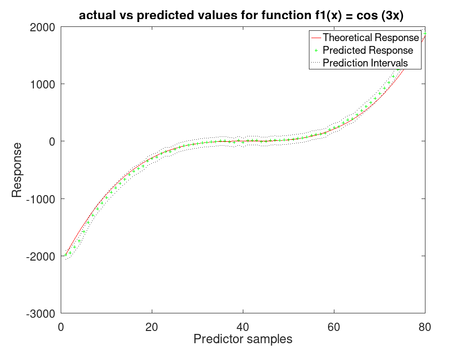
Plot the results

 figure
 [sortedY, indY] = sort (Ytrue(test (C)));
 plot (sortedY, 'r-');
 xlim ([0, sum(test(C))]);
 hold on
 plot (ypred(indY), 'g+')
 plot (yInt(indY,1),'k:')
 plot (yInt(indY,2),'k:')
 xlabel ('Predictor samples');
 ylabel ('Response');
 title ('actual vs predicted values for function f1(x) = cos (3x) ');
 legend ({'Theoretical Response', 'Predicted Response', 'Prediction Intervals'});

A cell array with one row vector per predictor, holding the coarse cut points the residuals of the predictor phase were laid on while pairs were being tested. The grid is eight equal-frequency bins whatever the sample size, as MATLAB’s is. It is empty when the model carries no interaction terms, and empty throughout under the spline engine, which does not bin.

This property is read-only.

Train a RegressionGAM Model for synthetic values

 rng (42);
 f1 = @(x) cos (3 * x);
 f2 = @(x) x .^ 3;
 x1 = 2 * rand (50, 1) - 1;
 x2 = 2 * rand (50, 1) - 1;
 y = f1(x1) + f2(x2);
 y = y + y .* 0.2 .* rand (50,1);
 X = [x1, x2];
 a = fitrgam (X, y)

a =

  RegressionGAM

             ResponseName: 'Y'
          NumObservations: 50
            NumPredictors: 2
        ResponseTransform: 'none'
                Intercept: 0.0671178
                    Knots: []
                    Order: []
                      Tol:

Declare two different functions

 rng (42);
 f1 = @(x) cos (3 * x);
 f2 = @(x) x .^ 3;

Generate 80 samples for f1 and f2

 x = [-4*pi:0.1*pi:4*pi-0.1*pi]';
 X1 = f1(x);
 X2 = f2(x);

Create a synthetic response by adding noise

 Ytrue = X1 + X2;
 Y = Ytrue + Ytrue .* 0.2 .* rand (80,1);

Assemble predictor data

 X = [X1, X2];

Train the GAM and test on the same data A standard deviation and a prediction interval come from the spline engine, which fits one; the boosted-tree engine reports none.

 a = fitrgam (X, Y, 'FitMethod', 'splines', 'order', [5, 5]);
 [ypred, ySDsd, yInt] = predict (a, X);

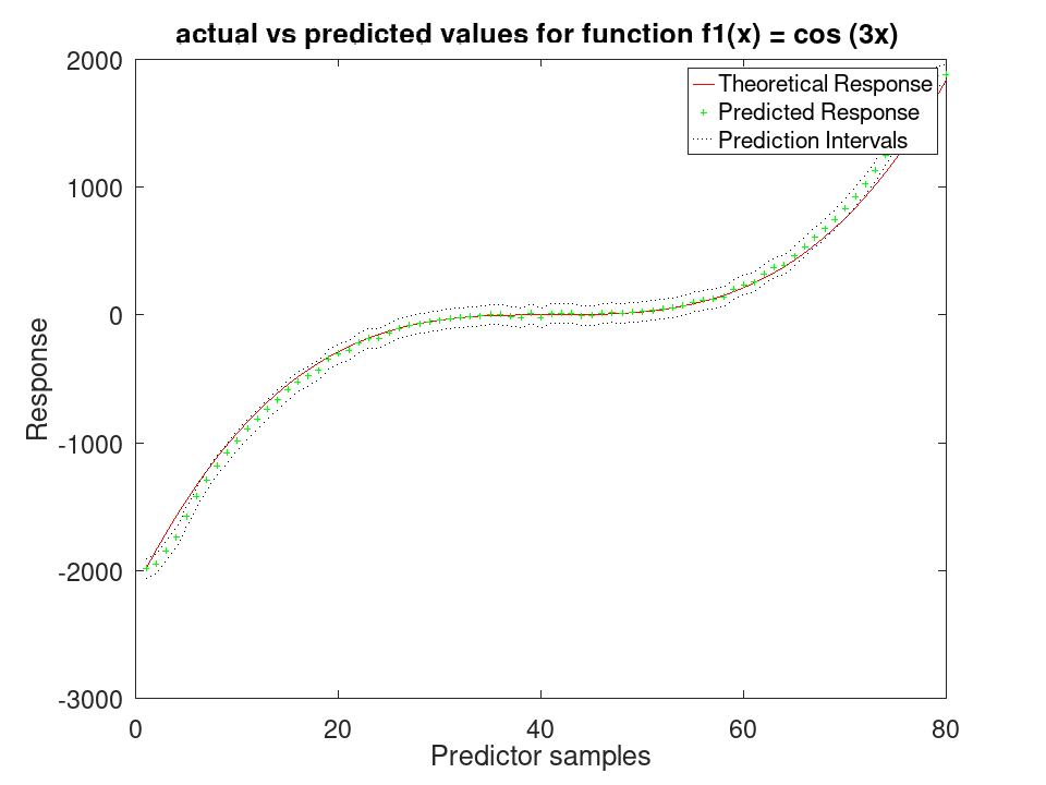
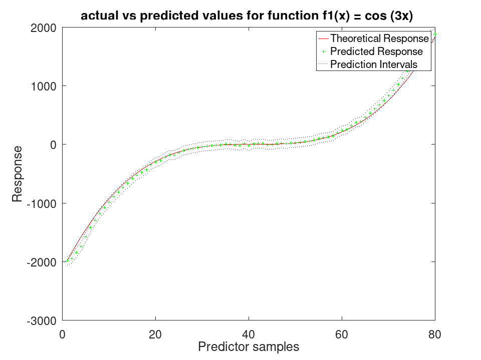
Plot the results

 figure
 [sortedY, indY] = sort (Ytrue);
 plot (sortedY, 'r-');
 xlim ([0, 80]);
 hold on
 plot (ypred(indY), 'g+')
 plot (yInt(indY,1), 'k:')
 plot (yInt(indY,2), 'k:')
 xlabel ('Predictor samples');
 ylabel ('Response');
 title ('actual vs predicted values for function f1(x) = cos (3x) ');
 legend ({'Theoretical Response', 'Predicted Response', 'Prediction Intervals'});

Use 30% Holdout partitioning for training and testing data

 C = cvpartition (80, 'HoldOut', 0.3);
 [ypred, ySDsd, yInt] = predict (a, X(test (C),:));

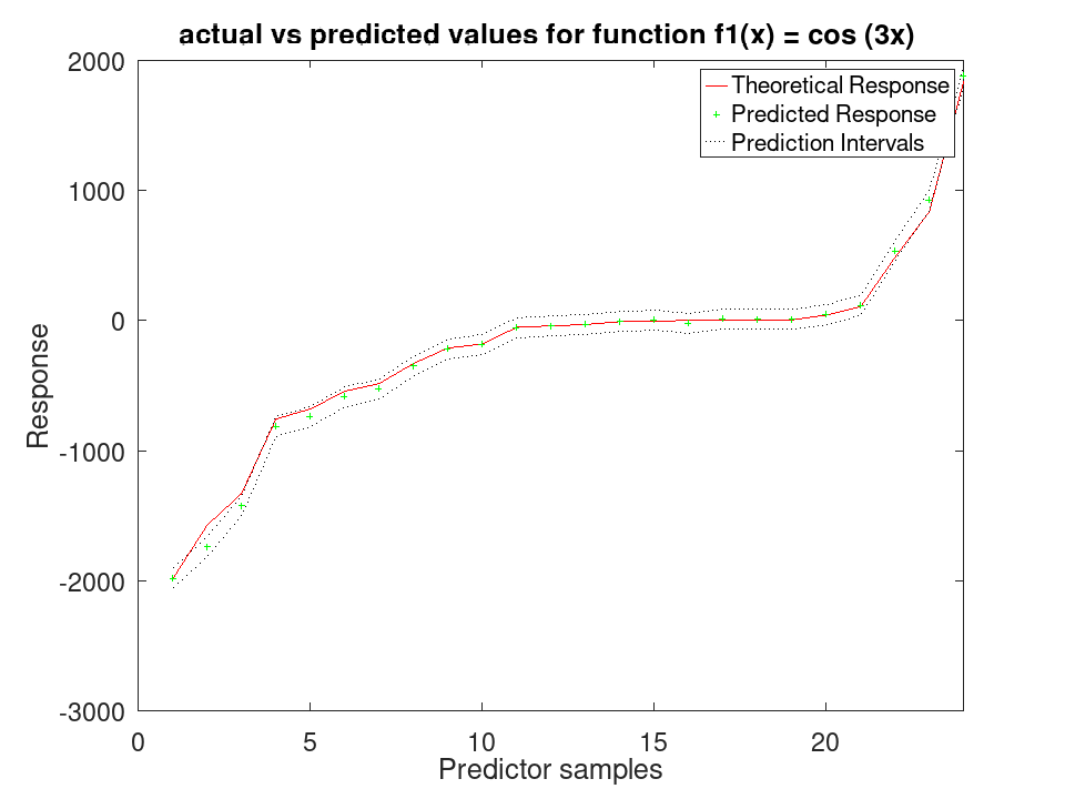
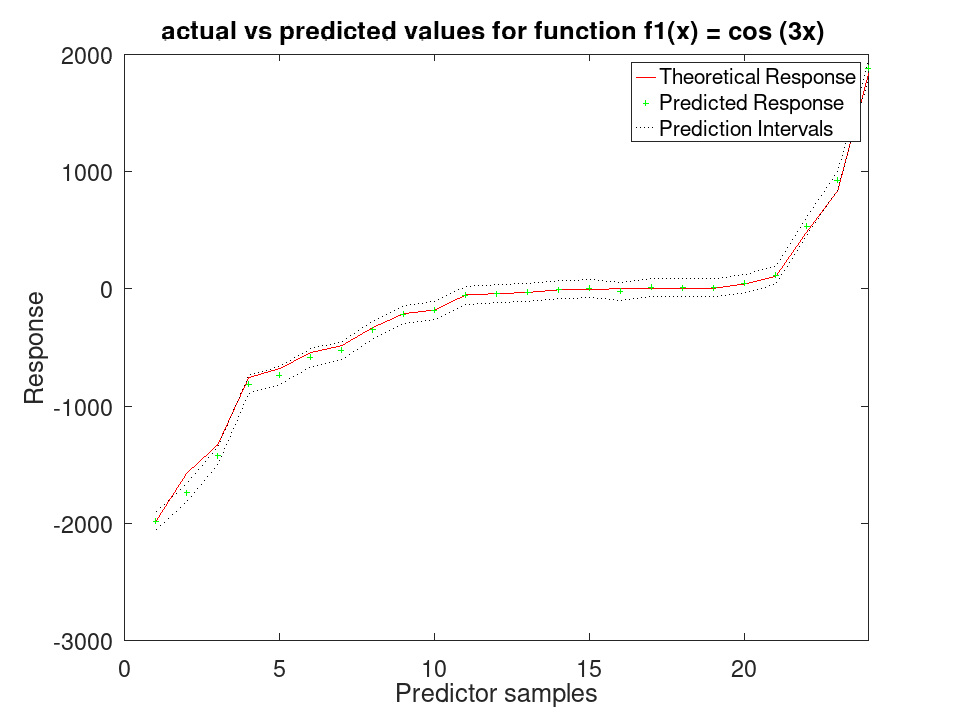
Plot the results

 figure
 [sortedY, indY] = sort (Ytrue(test (C)));
 plot (sortedY, 'r-');
 xlim ([0, sum(test(C))]);
 hold on
 plot (ypred(indY), 'g+')
 plot (yInt(indY,1),'k:')
 plot (yInt(indY,2),'k:')
 xlabel ('Predictor samples');
 ylabel ('Response');
 title ('actual vs predicted values for function f1(x) = cos (3x) ');
 legend ({'Theoretical Response', 'Predicted Response', 'Prediction Intervals'});

A structure holding the fitting parameters. Under the boosted-tree engine it carries MATLAB’s own fields, with Type reading 'regression'; under the spline engine it describes that scheme instead, since none of the tree vocabulary applies to it.

This property is read-only.

Train a RegressionGAM Model for synthetic values

 rng (42);
 f1 = @(x) cos (3 * x);
 f2 = @(x) x .^ 3;
 x1 = 2 * rand (50, 1) - 1;
 x2 = 2 * rand (50, 1) - 1;
 y = f1(x1) + f2(x2);
 y = y + y .* 0.2 .* rand (50,1);
 X = [x1, x2];
 a = fitrgam (X, y)

a =

  RegressionGAM

             ResponseName: 'Y'
          NumObservations: 50
            NumPredictors: 2
        ResponseTransform: 'none'
                Intercept: 0.0671178
                    Knots: []
                    Order: []
                      Tol:

Declare two different functions

 rng (42);
 f1 = @(x) cos (3 * x);
 f2 = @(x) x .^ 3;

Generate 80 samples for f1 and f2

 x = [-4*pi:0.1*pi:4*pi-0.1*pi]';
 X1 = f1(x);
 X2 = f2(x);

Create a synthetic response by adding noise

 Ytrue = X1 + X2;
 Y = Ytrue + Ytrue .* 0.2 .* rand (80,1);

Assemble predictor data

 X = [X1, X2];

Train the GAM and test on the same data A standard deviation and a prediction interval come from the spline engine, which fits one; the boosted-tree engine reports none.

 a = fitrgam (X, Y, 'FitMethod', 'splines', 'order', [5, 5]);
 [ypred, ySDsd, yInt] = predict (a, X);

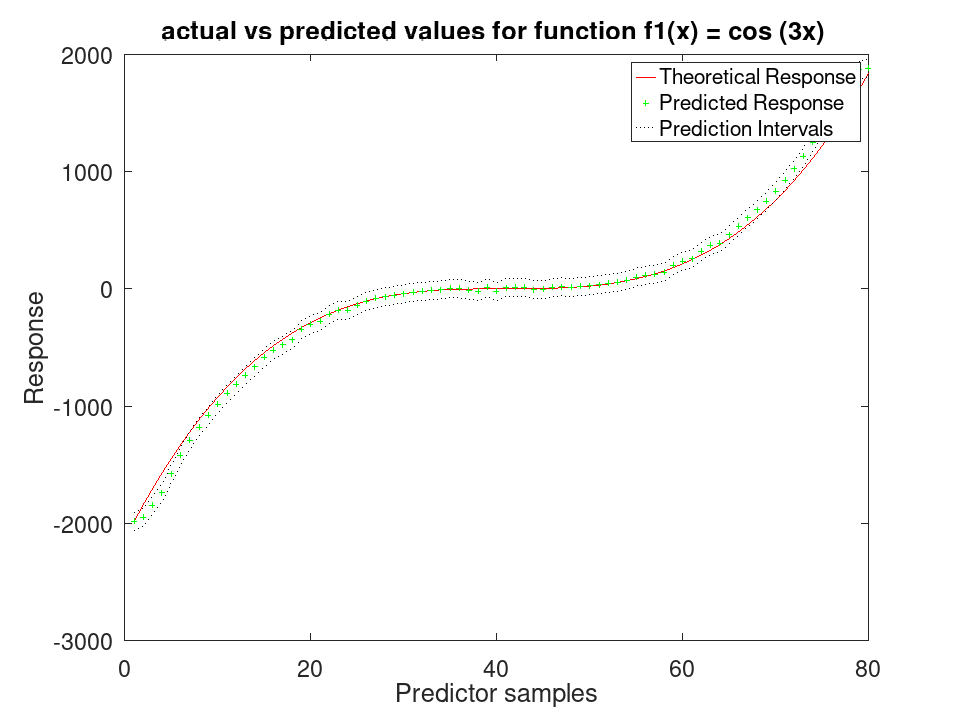
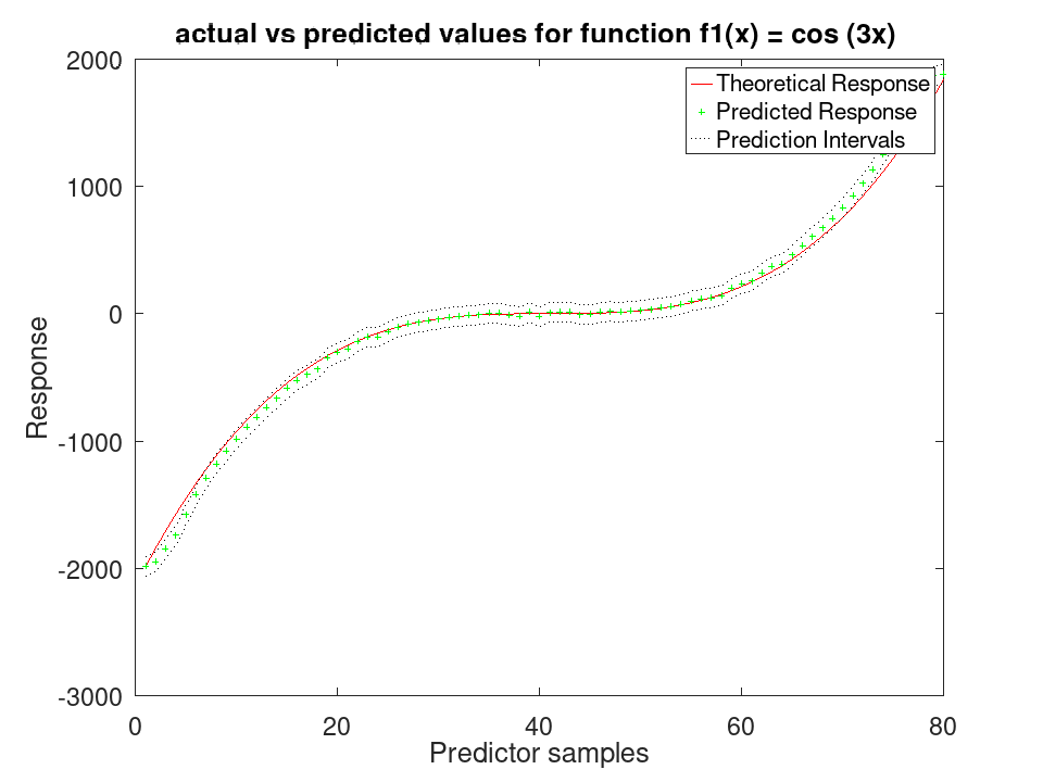
Plot the results

 figure
 [sortedY, indY] = sort (Ytrue);
 plot (sortedY, 'r-');
 xlim ([0, 80]);
 hold on
 plot (ypred(indY), 'g+')
 plot (yInt(indY,1), 'k:')
 plot (yInt(indY,2), 'k:')
 xlabel ('Predictor samples');
 ylabel ('Response');
 title ('actual vs predicted values for function f1(x) = cos (3x) ');
 legend ({'Theoretical Response', 'Predicted Response', 'Prediction Intervals'});

Use 30% Holdout partitioning for training and testing data

 C = cvpartition (80, 'HoldOut', 0.3);
 [ypred, ySDsd, yInt] = predict (a, X(test (C),:));

Plot the results

 figure
 [sortedY, indY] = sort (Ytrue(test (C)));
 plot (sortedY, 'r-');
 xlim ([0, sum(test(C))]);
 hold on
 plot (ypred(indY), 'g+')
 plot (yInt(indY,1),'k:')
 plot (yInt(indY,2),'k:')
 xlabel ('Predictor samples');
 ylabel ('Response');
 title ('actual vs predicted values for function f1(x) = cos (3x) ');
 legend ({'Theoretical Response', 'Predicted Response', 'Prediction Intervals'});

A structure with the fields PredictorTrees and InteractionTrees, each saying why that phase ended. A phase that never ran reports an empty character vector. It is empty under the spline engine, which has no tree budget to exhaust.

This property is read-only.

Train a RegressionGAM Model for synthetic values

 rng (42);
 f1 = @(x) cos (3 * x);
 f2 = @(x) x .^ 3;
 x1 = 2 * rand (50, 1) - 1;
 x2 = 2 * rand (50, 1) - 1;
 y = f1(x1) + f2(x2);
 y = y + y .* 0.2 .* rand (50,1);
 X = [x1, x2];
 a = fitrgam (X, y)

a =

  RegressionGAM

             ResponseName: 'Y'
          NumObservations: 50
            NumPredictors: 2
        ResponseTransform: 'none'
                Intercept: 0.0671178
                    Knots: []
                    Order: []
                      Tol:

Declare two different functions

 rng (42);
 f1 = @(x) cos (3 * x);
 f2 = @(x) x .^ 3;

Generate 80 samples for f1 and f2

 x = [-4*pi:0.1*pi:4*pi-0.1*pi]';
 X1 = f1(x);
 X2 = f2(x);

Create a synthetic response by adding noise

 Ytrue = X1 + X2;
 Y = Ytrue + Ytrue .* 0.2 .* rand (80,1);

Assemble predictor data

 X = [X1, X2];

Train the GAM and test on the same data A standard deviation and a prediction interval come from the spline engine, which fits one; the boosted-tree engine reports none.

 a = fitrgam (X, Y, 'FitMethod', 'splines', 'order', [5, 5]);
 [ypred, ySDsd, yInt] = predict (a, X);

Plot the results

 figure
 [sortedY, indY] = sort (Ytrue);
 plot (sortedY, 'r-');
 xlim ([0, 80]);
 hold on
 plot (ypred(indY), 'g+')
 plot (yInt(indY,1), 'k:')
 plot (yInt(indY,2), 'k:')
 xlabel ('Predictor samples');
 ylabel ('Response');
 title ('actual vs predicted values for function f1(x) = cos (3x) ');
 legend ({'Theoretical Response', 'Predicted Response', 'Prediction Intervals'});

Use 30% Holdout partitioning for training and testing data

 C = cvpartition (80, 'HoldOut', 0.3);
 [ypred, ySDsd, yInt] = predict (a, X(test (C),:));

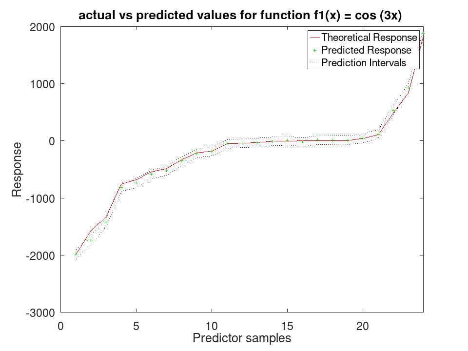
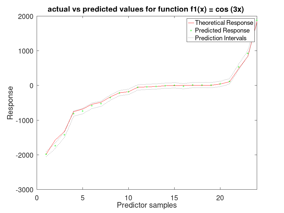
Plot the results

 figure
 [sortedY, indY] = sort (Ytrue(test (C)));
 plot (sortedY, 'r-');
 xlim ([0, sum(test(C))]);
 hold on
 plot (ypred(indY), 'g+')
 plot (yInt(indY,1),'k:')
 plot (yInt(indY,2),'k:')
 xlabel ('Predictor samples');
 ylabel ('Response');
 title ('actual vs predicted values for function f1(x) = cos (3x) ');
 legend ({'Theoretical Response', 'Predicted Response', 'Prediction Intervals'});

A character vector, either 'boostedtrees' or 'splines'. The default is 'boostedtrees', the scheme MATLAB’s generalized additive model uses. 'splines' selects the penalised-spline engine, an Octave extension with no MATLAB counterpart and the scheme this class fitted before version 1.9.0. The two engines take different arguments and an argument meant for one is refused by the other rather than ignored.

This property is read-only.

Train a RegressionGAM Model for synthetic values

 rng (42);
 f1 = @(x) cos (3 * x);
 f2 = @(x) x .^ 3;
 x1 = 2 * rand (50, 1) - 1;
 x2 = 2 * rand (50, 1) - 1;
 y = f1(x1) + f2(x2);
 y = y + y .* 0.2 .* rand (50,1);
 X = [x1, x2];
 a = fitrgam (X, y)

a =

  RegressionGAM

             ResponseName: 'Y'
          NumObservations: 50
            NumPredictors: 2
        ResponseTransform: 'none'
                Intercept: 0.0671178
                    Knots: []
                    Order: []
                      Tol:

Declare two different functions

 rng (42);
 f1 = @(x) cos (3 * x);
 f2 = @(x) x .^ 3;

Generate 80 samples for f1 and f2

 x = [-4*pi:0.1*pi:4*pi-0.1*pi]';
 X1 = f1(x);
 X2 = f2(x);

Create a synthetic response by adding noise

 Ytrue = X1 + X2;
 Y = Ytrue + Ytrue .* 0.2 .* rand (80,1);

Assemble predictor data

 X = [X1, X2];

Train the GAM and test on the same data A standard deviation and a prediction interval come from the spline engine, which fits one; the boosted-tree engine reports none.

 a = fitrgam (X, Y, 'FitMethod', 'splines', 'order', [5, 5]);
 [ypred, ySDsd, yInt] = predict (a, X);

Plot the results

 figure
 [sortedY, indY] = sort (Ytrue);
 plot (sortedY, 'r-');
 xlim ([0, 80]);
 hold on
 plot (ypred(indY), 'g+')
 plot (yInt(indY,1), 'k:')
 plot (yInt(indY,2), 'k:')
 xlabel ('Predictor samples');
 ylabel ('Response');
 title ('actual vs predicted values for function f1(x) = cos (3x) ');
 legend ({'Theoretical Response', 'Predicted Response', 'Prediction Intervals'});

Use 30% Holdout partitioning for training and testing data

 C = cvpartition (80, 'HoldOut', 0.3);
 [ypred, ySDsd, yInt] = predict (a, X(test (C),:));

Plot the results

 figure
 [sortedY, indY] = sort (Ytrue(test (C)));
 plot (sortedY, 'r-');
 xlim ([0, sum(test(C))]);
 hold on
 plot (ypred(indY), 'g+')
 plot (yInt(indY,1),'k:')
 plot (yInt(indY,2),'k:')
 xlabel ('Predictor samples');
 ylabel ('Response');
 title ('actual vs predicted values for function f1(x) = cos (3x) ');
 legend ({'Theoretical Response', 'Predicted Response', 'Prediction Intervals'});

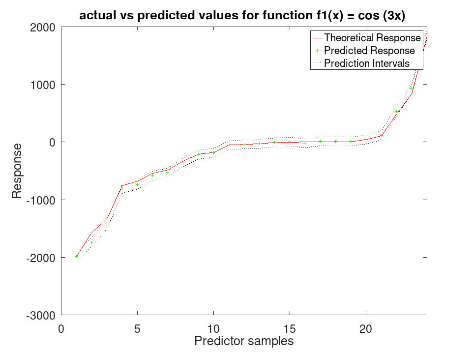
A structure with fields ShapeValues, PairValues and Pairs, holding what the boosted-tree engine fitted. MATLAB exposes no equivalent, reporting its bin edges but never the values on them, so this is an Octave extension. It is empty under the spline engine, whose fit lives in BaseModel and ModelwInt.

This property is read-only.

Train a RegressionGAM Model for synthetic values

 rng (42);
 f1 = @(x) cos (3 * x);
 f2 = @(x) x .^ 3;
 x1 = 2 * rand (50, 1) - 1;
 x2 = 2 * rand (50, 1) - 1;
 y = f1(x1) + f2(x2);
 y = y + y .* 0.2 .* rand (50,1);
 X = [x1, x2];
 a = fitrgam (X, y)

a =

  RegressionGAM

             ResponseName: 'Y'
          NumObservations: 50
            NumPredictors: 2
        ResponseTransform: 'none'
                Intercept: 0.0671178
                    Knots: []
                    Order: []
                      Tol:

Declare two different functions

 rng (42);
 f1 = @(x) cos (3 * x);
 f2 = @(x) x .^ 3;

Generate 80 samples for f1 and f2

 x = [-4*pi:0.1*pi:4*pi-0.1*pi]';
 X1 = f1(x);
 X2 = f2(x);

Create a synthetic response by adding noise

 Ytrue = X1 + X2;
 Y = Ytrue + Ytrue .* 0.2 .* rand (80,1);

Assemble predictor data

 X = [X1, X2];

Train the GAM and test on the same data A standard deviation and a prediction interval come from the spline engine, which fits one; the boosted-tree engine reports none.

 a = fitrgam (X, Y, 'FitMethod', 'splines', 'order', [5, 5]);
 [ypred, ySDsd, yInt] = predict (a, X);

Plot the results

 figure
 [sortedY, indY] = sort (Ytrue);
 plot (sortedY, 'r-');
 xlim ([0, 80]);
 hold on
 plot (ypred(indY), 'g+')
 plot (yInt(indY,1), 'k:')
 plot (yInt(indY,2), 'k:')
 xlabel ('Predictor samples');
 ylabel ('Response');
 title ('actual vs predicted values for function f1(x) = cos (3x) ');
 legend ({'Theoretical Response', 'Predicted Response', 'Prediction Intervals'});

Use 30% Holdout partitioning for training and testing data

 C = cvpartition (80, 'HoldOut', 0.3);
 [ypred, ySDsd, yInt] = predict (a, X(test (C),:));

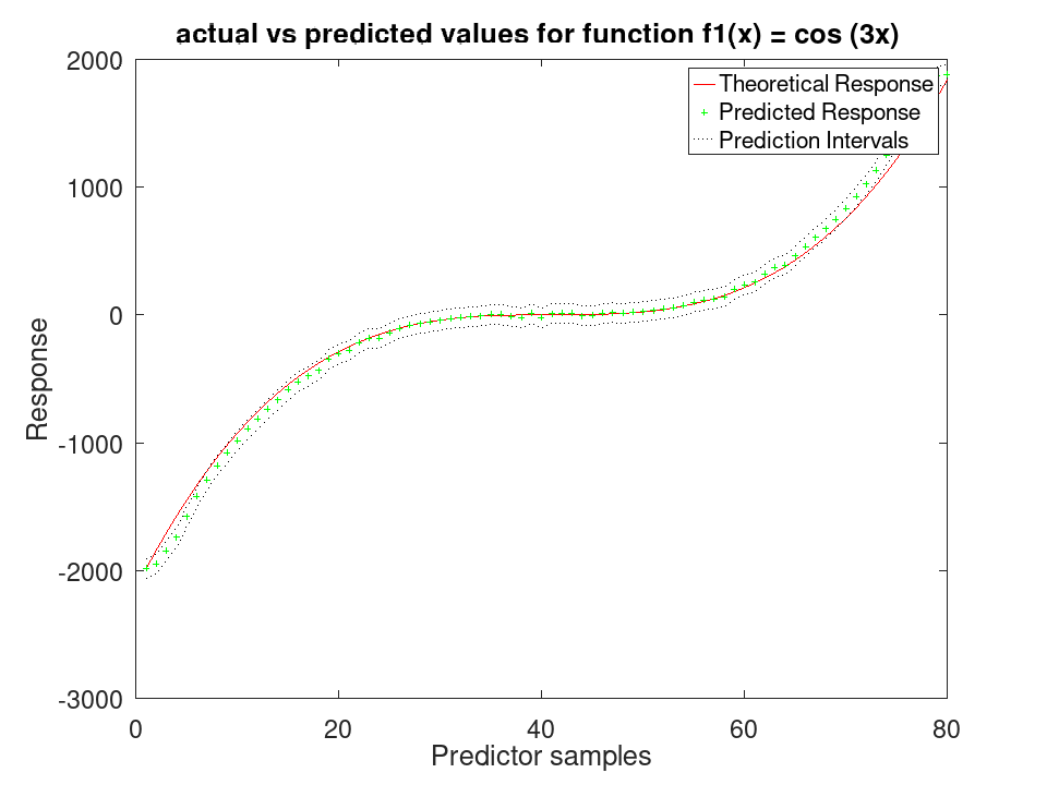
Plot the results

 figure
 [sortedY, indY] = sort (Ytrue(test (C)));
 plot (sortedY, 'r-');
 xlim ([0, sum(test(C))]);
 hold on
 plot (ypred(indY), 'g+')
 plot (yInt(indY,1),'k:')
 plot (yInt(indY,2),'k:')
 xlabel ('Predictor samples');
 ylabel ('Response');
 title ('actual vs predicted values for function f1(x) = cos (3x) ');
 legend ({'Theoretical Response', 'Predicted Response', 'Prediction Intervals'});

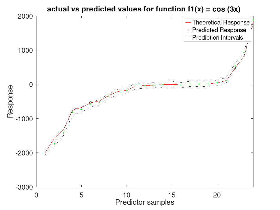
Always empty. It is declared for MATLAB compatibility, where it holds what an automatic search over the hyperparameters found. This class fits the parameters it is given and runs no such search, so there is nothing to report. This property is read-only.

Train a RegressionGAM Model for synthetic values

 rng (42);
 f1 = @(x) cos (3 * x);
 f2 = @(x) x .^ 3;
 x1 = 2 * rand (50, 1) - 1;
 x2 = 2 * rand (50, 1) - 1;
 y = f1(x1) + f2(x2);
 y = y + y .* 0.2 .* rand (50,1);
 X = [x1, x2];
 a = fitrgam (X, y)

a =

  RegressionGAM

             ResponseName: 'Y'
          NumObservations: 50
            NumPredictors: 2
        ResponseTransform: 'none'
                Intercept: 0.0671178
                    Knots: []
                    Order: []
                      Tol:

Declare two different functions

 rng (42);
 f1 = @(x) cos (3 * x);
 f2 = @(x) x .^ 3;

Generate 80 samples for f1 and f2

 x = [-4*pi:0.1*pi:4*pi-0.1*pi]';
 X1 = f1(x);
 X2 = f2(x);

Create a synthetic response by adding noise

 Ytrue = X1 + X2;
 Y = Ytrue + Ytrue .* 0.2 .* rand (80,1);

Assemble predictor data

 X = [X1, X2];

Train the GAM and test on the same data A standard deviation and a prediction interval come from the spline engine, which fits one; the boosted-tree engine reports none.

 a = fitrgam (X, Y, 'FitMethod', 'splines', 'order', [5, 5]);
 [ypred, ySDsd, yInt] = predict (a, X);

Plot the results

 figure
 [sortedY, indY] = sort (Ytrue);
 plot (sortedY, 'r-');
 xlim ([0, 80]);
 hold on
 plot (ypred(indY), 'g+')
 plot (yInt(indY,1), 'k:')
 plot (yInt(indY,2), 'k:')
 xlabel ('Predictor samples');
 ylabel ('Response');
 title ('actual vs predicted values for function f1(x) = cos (3x) ');
 legend ({'Theoretical Response', 'Predicted Response', 'Prediction Intervals'});

Use 30% Holdout partitioning for training and testing data

 C = cvpartition (80, 'HoldOut', 0.3);
 [ypred, ySDsd, yInt] = predict (a, X(test (C),:));

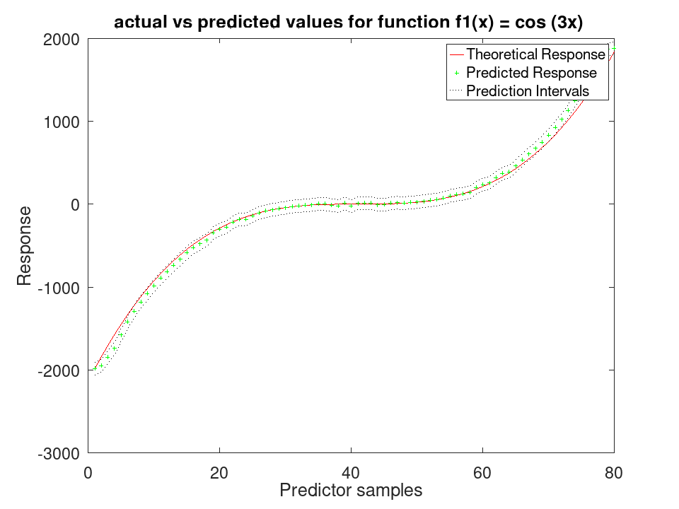
Plot the results

 figure
 [sortedY, indY] = sort (Ytrue(test (C)));
 plot (sortedY, 'r-');
 xlim ([0, sum(test(C))]);
 hold on
 plot (ypred(indY), 'g+')
 plot (yInt(indY,1),'k:')
 plot (yInt(indY,2),'k:')
 xlabel ('Predictor samples');
 ylabel ('Response');
 title ('actual vs predicted values for function f1(x) = cos (3x) ');
 legend ({'Theoretical Response', 'Predicted Response', 'Prediction Intervals'});

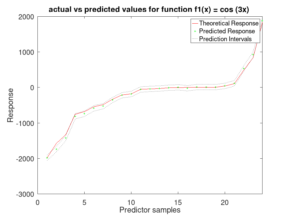
A function handle applied to the response the model predicts. Add or change it using dot notation, as in obj.ResponseTransform = 'log' or obj.ResponseTransform = @function_handle. It defaults to 'none', the identity.

Train a RegressionGAM Model for synthetic values

 rng (42);
 f1 = @(x) cos (3 * x);
 f2 = @(x) x .^ 3;
 x1 = 2 * rand (50, 1) - 1;
 x2 = 2 * rand (50, 1) - 1;
 y = f1(x1) + f2(x2);
 y = y + y .* 0.2 .* rand (50,1);
 X = [x1, x2];
 a = fitrgam (X, y)

a =

  RegressionGAM

             ResponseName: 'Y'
          NumObservations: 50
            NumPredictors: 2
        ResponseTransform: 'none'
                Intercept: 0.0671178
                    Knots: []
                    Order: []
                      Tol:

Declare two different functions

 rng (42);
 f1 = @(x) cos (3 * x);
 f2 = @(x) x .^ 3;

Generate 80 samples for f1 and f2

 x = [-4*pi:0.1*pi:4*pi-0.1*pi]';
 X1 = f1(x);
 X2 = f2(x);

Create a synthetic response by adding noise

 Ytrue = X1 + X2;
 Y = Ytrue + Ytrue .* 0.2 .* rand (80,1);

Assemble predictor data

 X = [X1, X2];

Train the GAM and test on the same data A standard deviation and a prediction interval come from the spline engine, which fits one; the boosted-tree engine reports none.

 a = fitrgam (X, Y, 'FitMethod', 'splines', 'order', [5, 5]);
 [ypred, ySDsd, yInt] = predict (a, X);

Plot the results

 figure
 [sortedY, indY] = sort (Ytrue);
 plot (sortedY, 'r-');
 xlim ([0, 80]);
 hold on
 plot (ypred(indY), 'g+')
 plot (yInt(indY,1), 'k:')
 plot (yInt(indY,2), 'k:')
 xlabel ('Predictor samples');
 ylabel ('Response');
 title ('actual vs predicted values for function f1(x) = cos (3x) ');
 legend ({'Theoretical Response', 'Predicted Response', 'Prediction Intervals'});

Use 30% Holdout partitioning for training and testing data

 C = cvpartition (80, 'HoldOut', 0.3);
 [ypred, ySDsd, yInt] = predict (a, X(test (C),:));

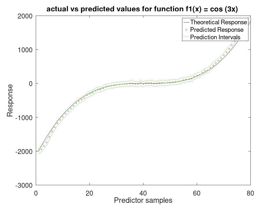
Plot the results

 figure
 [sortedY, indY] = sort (Ytrue(test (C)));
 plot (sortedY, 'r-');
 xlim ([0, sum(test(C))]);
 hold on
 plot (ypred(indY), 'g+')
 plot (yInt(indY,1),'k:')
 plot (yInt(indY,2),'k:')
 xlabel ('Predictor samples');
 ylabel ('Response');
 title ('actual vs predicted values for function f1(x) = cos (3x) ');
 legend ({'Theoretical Response', 'Predicted Response', 'Prediction Intervals'});

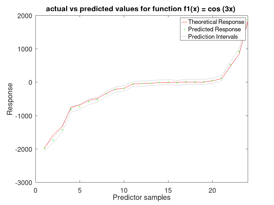
The RegressionGAM class offers the following public methods:

RegressionGAM: obj = RegressionGAM (X, Y)

RegressionGAM: obj = RegressionGAM (Tbl, ResponseVarName)

RegressionGAM: obj = RegressionGAM (Tbl, formula)

RegressionGAM: obj = RegressionGAM (Tbl, Y)

RegressionGAM: obj = RegressionGAM (…, name, value)

obj = RegressionGAM (X, Y) returns an object of class RegressionGAM, with matrix X containing the predictor data and vector Y containing the continuous response data.

X must be a N×P numeric matrix of input data where rows correspond to observations and columns correspond to features or variables. X will be used to train the GAM model.
Y must be N×1 numeric vector containing the response data corresponding to the predictor data in X. Y must have same number of rows as X.

obj = RegressionGAM (…, name, value) returns an object of class RegressionGAM with additional properties specified by Name-Value pair arguments listed below.

`Name`	`Value`
`'Predictors'`	Predictor Variable names, specified as a row vector cell of strings with the same length as the columns in `X`. If omitted, the program will generate default variable names `(x1, x2, ..., xn)` for each column in `X`.
`'responsename'`	Response Variable Name, specified as a string. If omitted, the default value is `'Y'`.
`'formula'`	(spline option) a model specification given as a string in the form `'Y ~ terms'` where `Y` represents the response variable and `terms` the predictor variables. The formula can be used to specify a subset of variables for training model. For example: `'Y ~ x1 + x2 + x3 + x4 + x1:x2 + x2:x3'` specifies four linear terms for the first four columns of for predictor data, and `x1:x2` and `x2:x3` specify the two interaction terms for 1st-2nd and 3rd-4th columns respectively. Only these terms will be used for training the model, but `X` must have at least as many columns as referenced in the formula. If Predictor Variable names have been defined, then the terms in the formula must reference to those. When `'formula'` is specified, all terms used for training the model are referenced in the `IntMatrix` field of the `obj` class object as a matrix containing the column indexes for each term including both the predictors and the interactions used.
`'interactions'`	a logical matrix, a positive integer scalar, or the string `'all'` for defining the interactions between predictor variables. When given a logical matrix, it must have the same number of columns as `X` and each row corresponds to a different interaction term combining the predictors indexed as `true`. Each interaction term is appended as a column vector after the available predictor column in `X`. When `'all'` is defined, then all possible combinations of interactions are appended in `X` before training. At the moment, parsing a positive integer has the same effect as the `'all'` option. When `'interactions'` is specified, only the interaction terms appended to `X` are referenced in the `IntMatrix` field of the `obj` class object.
`'knots'`	(spline option) a scalar or a row vector with the same columns as `X`. It defines the knots for fitting a polynomial when training the GAM. As a scalar, it is expanded to a row vector. The default value is 5, hence expanded to `ones (1, columns (X)) * 5`. You can parse a row vector with different number of knots for each predictor variable to be fitted with, although not recommended.
`'order'`	(spline option) a scalar or a row vector with the same columns as `X`. It defines the order of the polynomial when training the GAM. As a scalar, it is expanded to a row vector. The default values is 3, hence expanded to `ones (1, columns (X)) * 3`. You can parse a row vector with different number of polynomial order for each predictor variable to be fitted with, although not recommended.
`'dof'`	(spline option) a scalar or a row vector with the same columns as `X`. It defines the degrees of freedom for fitting a polynomial when training the GAM. As a scalar, it is expanded to a row vector. The default value is 8, hence expanded to `ones (1, columns (X)) * 8`. You can parse a row vector with different degrees of freedom for each predictor variable to be fitted with, although not recommended.
`'tol'`	(spline option) a positive scalar to set the tolerance for convergence during training. By default, it is set to `1e-3`.

A row marked (spline option) belongs to the spline engine and requires 'FitMethod', 'splines'; passing one under the default boosted-tree engine is an error rather than being ignored. The boosted-tree engine’s own options are documented under fitrgam.

You can parse either a 'formula' or an 'interactions' optional parameter. Parsing both parameters will result an error. Accordingly, you can only pass up to two parameters among 'knots', 'order', and 'dof' to define the required polynomial for training the GAM model.

Two weak learners are available, selected by FitMethod.

'boostedtrees', the default, boosts one shallow decision tree per predictor in each round, which is the scheme MATLAB’s generalized additive model uses. A second phase then boosts trees over pairs of predictors, where interactions are asked for.

'splines' boosts a smoothing spline per predictor until the residual sum of squares changes by less than 'Tol'. It has no MATLAB counterpart and is an Octave extension, kept because a smooth additive fit is a genuinely different and often better answer than a staircase of stumps. A standard deviation and a prediction interval are available from it alone.

The two take different arguments, and an argument meant for one is refused by the other rather than ignored.

The choice is visible in the properties. Knots, Order, DoF, Formula, Tol, BaseModel, ModelwInt and IntMatrix describe a spline fit and are empty under the boosted-tree engine, while ModelParameters, ReasonForTermination, BinEdges, PairDetectionBinEdges and TreeModel describe a tree fit and are empty under the spline engine.

Fitted values are not expected to equal MATLAB’s even under 'boostedtrees'. The stopping rule and the step-reduction limit are not recoverable from anything MATLAB reports, so this engine documents its own; what the two share is the estimator and the reported surface, not the arithmetic.

See also: fitrgam, regress, regress_gp

Train a RegressionGAM Model for synthetic values

 rng (42);
 f1 = @(x) cos (3 * x);
 f2 = @(x) x .^ 3;
 x1 = 2 * rand (50, 1) - 1;
 x2 = 2 * rand (50, 1) - 1;
 y = f1(x1) + f2(x2);
 y = y + y .* 0.2 .* rand (50,1);
 X = [x1, x2];
 a = fitrgam (X, y)

a =

  RegressionGAM

             ResponseName: 'Y'
          NumObservations: 50
            NumPredictors: 2
        ResponseTransform: 'none'
                Intercept: 0.0671178
                    Knots: []
                    Order: []
                      Tol:

Declare two different functions

 rng (42);
 f1 = @(x) cos (3 * x);
 f2 = @(x) x .^ 3;

Generate 80 samples for f1 and f2

 x = [-4*pi:0.1*pi:4*pi-0.1*pi]';
 X1 = f1(x);
 X2 = f2(x);

Create a synthetic response by adding noise

 Ytrue = X1 + X2;
 Y = Ytrue + Ytrue .* 0.2 .* rand (80,1);

Assemble predictor data

 X = [X1, X2];

Train the GAM and test on the same data A standard deviation and a prediction interval come from the spline engine, which fits one; the boosted-tree engine reports none.

 a = fitrgam (X, Y, 'FitMethod', 'splines', 'order', [5, 5]);
 [ypred, ySDsd, yInt] = predict (a, X);

Plot the results

 figure
 [sortedY, indY] = sort (Ytrue);
 plot (sortedY, 'r-');
 xlim ([0, 80]);
 hold on
 plot (ypred(indY), 'g+')
 plot (yInt(indY,1), 'k:')
 plot (yInt(indY,2), 'k:')
 xlabel ('Predictor samples');
 ylabel ('Response');
 title ('actual vs predicted values for function f1(x) = cos (3x) ');
 legend ({'Theoretical Response', 'Predicted Response', 'Prediction Intervals'});

Use 30% Holdout partitioning for training and testing data

 C = cvpartition (80, 'HoldOut', 0.3);
 [ypred, ySDsd, yInt] = predict (a, X(test (C),:));

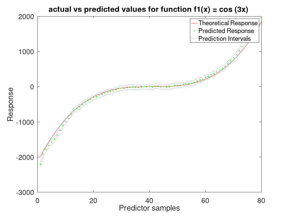
Plot the results

 figure
 [sortedY, indY] = sort (Ytrue(test (C)));
 plot (sortedY, 'r-');
 xlim ([0, sum(test(C))]);
 hold on
 plot (ypred(indY), 'g+')
 plot (yInt(indY,1),'k:')
 plot (yInt(indY,2),'k:')
 xlabel ('Predictor samples');
 ylabel ('Response');
 title ('actual vs predicted values for function f1(x) = cos (3x) ');
 legend ({'Theoretical Response', 'Predicted Response', 'Prediction Intervals'});

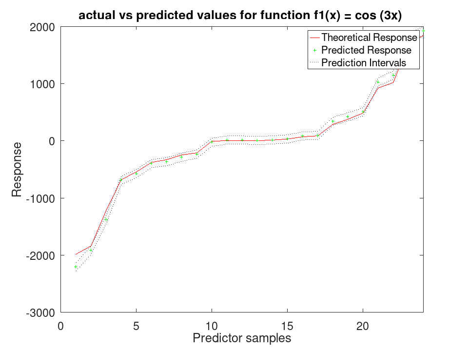
RegressionGAM: obj = addInteractions (obj, interactions)

obj = addInteractions (obj, interactions) fits the interaction terms named by interactions on top of the terms the model already carries and returns the updated model. The univariate fit is left alone, so predict with 'IncludeInteractions' set false answers exactly as it answered before.

interactions takes the forms the constructor’s 'Interactions' option takes: a nonnegative integer count of terms, a logical matrix with a column per predictor, or 'all'.

A model already carrying interaction terms is not extended, which is what MATLAB refuses too. A model fitted from a 'Formula' names every term it has, interactions among them, and is refused for the same reason.

Which terms a count selects is this implementation’s own: they are taken in the order nchoosek lists the pairs, where MATLAB ranks them by how much each contributes. The constructor’s option chooses the same way, so the two agree with each other.

See also: fitrgam, RegressionGAM

Train a RegressionGAM Model for synthetic values

 rng (42);
 f1 = @(x) cos (3 * x);
 f2 = @(x) x .^ 3;
 x1 = 2 * rand (50, 1) - 1;
 x2 = 2 * rand (50, 1) - 1;
 y = f1(x1) + f2(x2);
 y = y + y .* 0.2 .* rand (50,1);
 X = [x1, x2];
 a = fitrgam (X, y)

a =

  RegressionGAM

             ResponseName: 'Y'
          NumObservations: 50
            NumPredictors: 2
        ResponseTransform: 'none'
                Intercept: 0.0671178
                    Knots: []
                    Order: []
                      Tol:

Declare two different functions

 rng (42);
 f1 = @(x) cos (3 * x);
 f2 = @(x) x .^ 3;

Generate 80 samples for f1 and f2

 x = [-4*pi:0.1*pi:4*pi-0.1*pi]';
 X1 = f1(x);
 X2 = f2(x);

Create a synthetic response by adding noise

 Ytrue = X1 + X2;
 Y = Ytrue + Ytrue .* 0.2 .* rand (80,1);

Assemble predictor data

 X = [X1, X2];

Train the GAM and test on the same data A standard deviation and a prediction interval come from the spline engine, which fits one; the boosted-tree engine reports none.

 a = fitrgam (X, Y, 'FitMethod', 'splines', 'order', [5, 5]);
 [ypred, ySDsd, yInt] = predict (a, X);

Plot the results

 figure
 [sortedY, indY] = sort (Ytrue);
 plot (sortedY, 'r-');
 xlim ([0, 80]);
 hold on
 plot (ypred(indY), 'g+')
 plot (yInt(indY,1), 'k:')
 plot (yInt(indY,2), 'k:')
 xlabel ('Predictor samples');
 ylabel ('Response');
 title ('actual vs predicted values for function f1(x) = cos (3x) ');
 legend ({'Theoretical Response', 'Predicted Response', 'Prediction Intervals'});

Use 30% Holdout partitioning for training and testing data

 C = cvpartition (80, 'HoldOut', 0.3);
 [ypred, ySDsd, yInt] = predict (a, X(test (C),:));

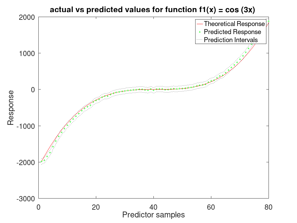
Plot the results

 figure
 [sortedY, indY] = sort (Ytrue(test (C)));
 plot (sortedY, 'r-');
 xlim ([0, sum(test(C))]);
 hold on
 plot (ypred(indY), 'g+')
 plot (yInt(indY,1),'k:')
 plot (yInt(indY,2),'k:')
 xlabel ('Predictor samples');
 ylabel ('Response');
 title ('actual vs predicted values for function f1(x) = cos (3x) ');
 legend ({'Theoretical Response', 'Predicted Response', 'Prediction Intervals'});

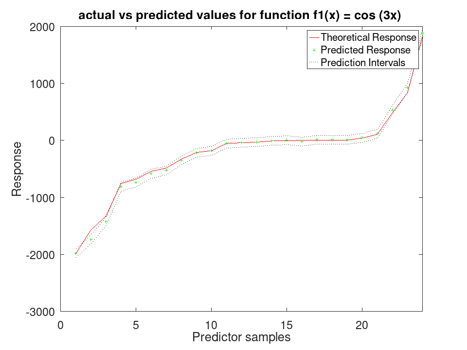
RegressionGAM: yFit = predict (obj, Xfit)

RegressionGAM: yFit = predict (…, Name, Value)

RegressionGAM: [yFit, ySD, yInt] = predict (…)

yFit = predict (obj, Xfit returns a vector of predicted responses, yFit, for the predictor data in matrix Xfit based on the Generalized Additive Model in obj. Xfit must have the same number of features/variables as the training data in obj. Every row is predicted. Under boosted trees a missing value adds nothing from a main effect, and an interaction term takes the value its trees give a row missing that predictor, so a row missing every predictor predicts the intercept; under splines a row holding a missing value is predicted as NaN.

obj must be a RegressionGAM class object.

[yFit, ySD, yInt] = predict (obj, Xfit also returns the standard deviations, ySD, and prediction intervals, yInt, of the response variable yFit, evaluated at each observation in the predictor data Xfit.

yFit = predict (…, Name, Value) returns the aforementioned results with additional properties specified by Name-Value pair arguments listed below.

`Name`	`Value`
`'alpha'`	significance level of the prediction intervals `yInt`, specified as scalar in range `[0,1]`. The default value is 0.05, which corresponds to 95% prediction intervals.
`'includeinteractions'`	a boolean flag to include interactions to predict new values based on `Xfit`. By default, `'includeinteractions'` is `true` when the GAM model in `obj` contains a `obj.Formula` or `obj.Interactions` fields. Otherwise, is set to `false`. If set to `true` when no interactions are present in the trained model, it will result to an error. If set to `false` when using a model that includes interactions, the predictions will be made on the basic model without any interaction terms. This way you can make predictions from the same GAM model without having to retrain it.

The new data may be a table, whose variables are matched to the predictors the model was fitted on by name and not by position: one the model was not fitted on is passed over, one it needs and cannot find is named, and a value holding a level is coded as that level was coded at fitting.

See also: fitrgam, RegressionGAM

Train a RegressionGAM Model for synthetic values

 rng (42);
 f1 = @(x) cos (3 * x);
 f2 = @(x) x .^ 3;
 x1 = 2 * rand (50, 1) - 1;
 x2 = 2 * rand (50, 1) - 1;
 y = f1(x1) + f2(x2);
 y = y + y .* 0.2 .* rand (50,1);
 X = [x1, x2];
 a = fitrgam (X, y)

a =

  RegressionGAM

             ResponseName: 'Y'
          NumObservations: 50
            NumPredictors: 2
        ResponseTransform: 'none'
                Intercept: 0.0671178
                    Knots: []
                    Order: []
                      Tol:

Declare two different functions

 rng (42);
 f1 = @(x) cos (3 * x);
 f2 = @(x) x .^ 3;

Generate 80 samples for f1 and f2

 x = [-4*pi:0.1*pi:4*pi-0.1*pi]';
 X1 = f1(x);
 X2 = f2(x);

Create a synthetic response by adding noise

 Ytrue = X1 + X2;
 Y = Ytrue + Ytrue .* 0.2 .* rand (80,1);

Assemble predictor data

 X = [X1, X2];

Train the GAM and test on the same data A standard deviation and a prediction interval come from the spline engine, which fits one; the boosted-tree engine reports none.

 a = fitrgam (X, Y, 'FitMethod', 'splines', 'order', [5, 5]);
 [ypred, ySDsd, yInt] = predict (a, X);

Plot the results

 figure
 [sortedY, indY] = sort (Ytrue);
 plot (sortedY, 'r-');
 xlim ([0, 80]);
 hold on
 plot (ypred(indY), 'g+')
 plot (yInt(indY,1), 'k:')
 plot (yInt(indY,2), 'k:')
 xlabel ('Predictor samples');
 ylabel ('Response');
 title ('actual vs predicted values for function f1(x) = cos (3x) ');
 legend ({'Theoretical Response', 'Predicted Response', 'Prediction Intervals'});

Use 30% Holdout partitioning for training and testing data

 C = cvpartition (80, 'HoldOut', 0.3);
 [ypred, ySDsd, yInt] = predict (a, X(test (C),:));

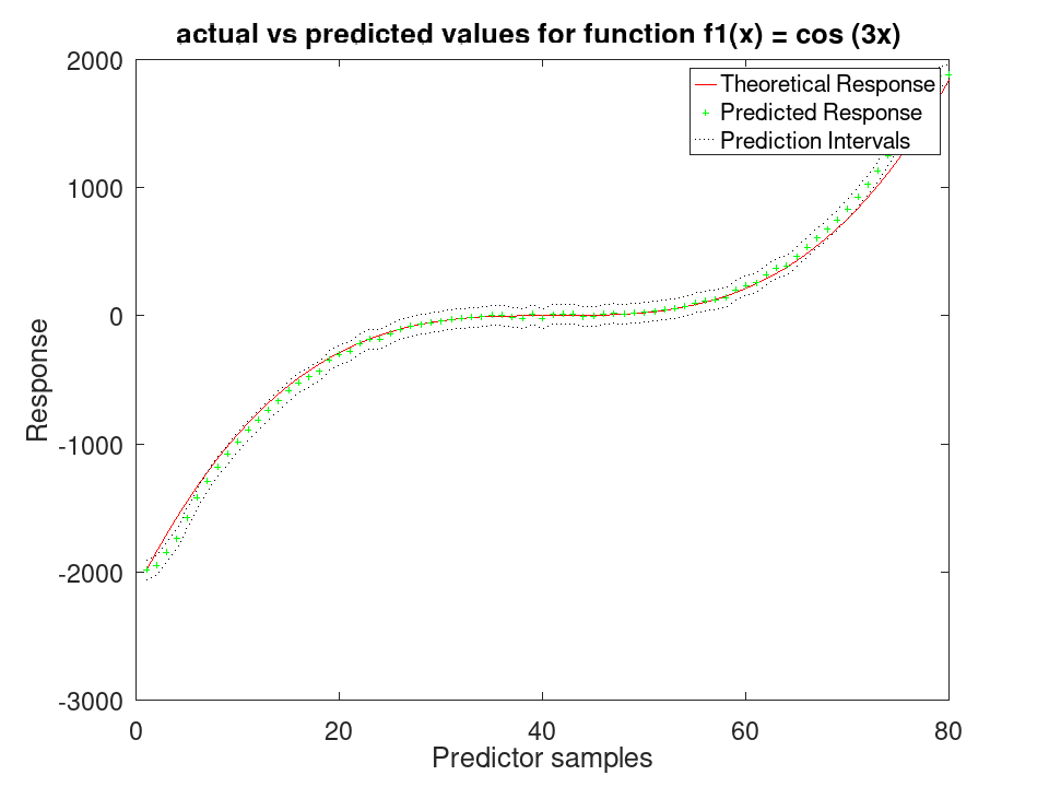
Plot the results

 figure
 [sortedY, indY] = sort (Ytrue(test (C)));
 plot (sortedY, 'r-');
 xlim ([0, sum(test(C))]);
 hold on
 plot (ypred(indY), 'g+')
 plot (yInt(indY,1),'k:')
 plot (yInt(indY,2),'k:')
 xlabel ('Predictor samples');
 ylabel ('Response');
 title ('actual vs predicted values for function f1(x) = cos (3x) ');
 legend ({'Theoretical Response', 'Predicted Response', 'Prediction Intervals'});

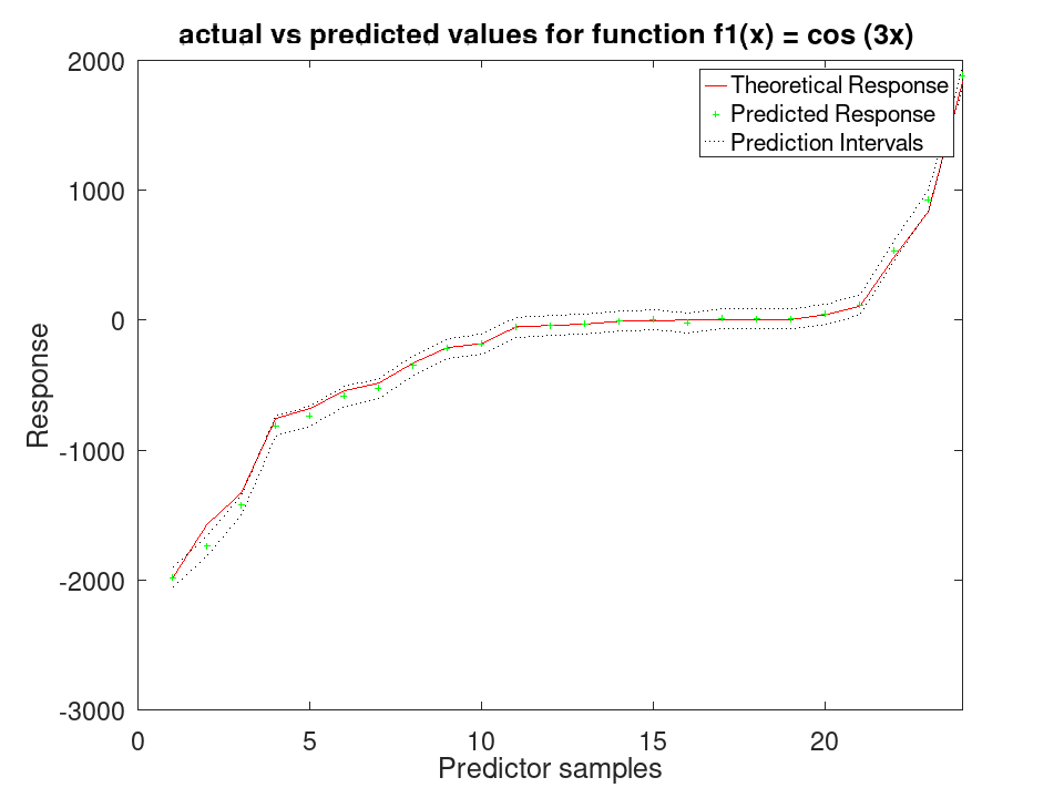
RegressionGAM: L = loss (obj, X, Y)

RegressionGAM: L = loss (obj, Tbl, ResponseVarName)

RegressionGAM: L = loss (obj, Tbl)

RegressionGAM: L = loss (…, name, value)

L = loss (obj, X, Y) returns the weighted mean squared error of the model on the rows of X against the true response Y.

X may also be a table Tbl, whose variables are matched to the predictors the model was fitted on by name and not by position. loss (obj, Tbl, ResponseVarName) takes the response from the variable ResponseVarName names, and loss (obj, Tbl) from the variable the model was fitted on. The response may also be given beside the table as Y.

L = loss (…, name, value) accepts the following name-value pairs:

"LossFun" selects the loss, either "mse", the default, or a function handle taking the true response, the predicted response and the weights, and returning a numeric scalar.
"Weights" holds one weight per row of X, normalised to sum to one before it is applied.

See also: RegressionGAM, fitrgam, RegressionGAM.predict

The mean squared error of the model on its own training data

 load fisheriris
 X = meas(:,1:3);
 Y = meas(:,4);
 mdl = fitrgam (X, Y);

resubLoss asks the same question without handing the data back in

 [loss(mdl, X, Y), resubLoss(mdl)]

ans =

   0.016330   0.016330

Interaction terms lower the loss on this data

 load fisheriris
 X = meas(:,1:3);
 Y = meas(:,4);

'all' fits every pairwise term on top of the additive ones

 [resubLoss(fitrgam (X, Y)), resubLoss(fitrgam (X, Y, 'Interactions', 'all'))]

ans =

   1.6330e-02   1.3237e-03

A loss function of your own, taking the truth, the fit and the weights

 load fisheriris
 X = meas(:,1:3);
 Y = meas(:,4);
 mdl = fitrgam (X, Y);

Mean absolute error instead of mean squared error

 mae = @(y, yfit, w) sum (w .* abs (y - yfit));
 [loss(mdl, X, Y), loss(mdl, X, Y, 'LossFun', mae)]

ans =

   0.016330   0.095652

Scoring a table

 load fisheriris
 T = table (meas(:,2), meas(:,3), meas(:,4), meas(:,1), ...
            'VariableNames', {'SW', 'PL', 'PW', 'SL'});
 mdl = fitrgam (T, 'SL');

The response is named by its column, left out, when it is the variable the model was fitted on, or given beside the predictors

 [loss(mdl, T, 'SL'), loss(mdl, T), loss(mdl, T(:, 1:3), T.SL)]

ans =

   0.049607   0.049607   0.049607

RegressionGAM: yFit = resubPredict (obj)

yFit = resubPredict (obj) is predict applied to the observations the model was fitted on.

See also: RegressionGAM, fitrgam, RegressionGAM.predict

Train a RegressionGAM Model for synthetic values

 rng (42);
 f1 = @(x) cos (3 * x);
 f2 = @(x) x .^ 3;
 x1 = 2 * rand (50, 1) - 1;
 x2 = 2 * rand (50, 1) - 1;
 y = f1(x1) + f2(x2);
 y = y + y .* 0.2 .* rand (50,1);
 X = [x1, x2];
 a = fitrgam (X, y)

a =

  RegressionGAM

             ResponseName: 'Y'
          NumObservations: 50
            NumPredictors: 2
        ResponseTransform: 'none'
                Intercept: 0.0671178
                    Knots: []
                    Order: []
                      Tol:

Declare two different functions

 rng (42);
 f1 = @(x) cos (3 * x);
 f2 = @(x) x .^ 3;

Generate 80 samples for f1 and f2

 x = [-4*pi:0.1*pi:4*pi-0.1*pi]';
 X1 = f1(x);
 X2 = f2(x);

Create a synthetic response by adding noise

 Ytrue = X1 + X2;
 Y = Ytrue + Ytrue .* 0.2 .* rand (80,1);

Assemble predictor data

 X = [X1, X2];

Train the GAM and test on the same data A standard deviation and a prediction interval come from the spline engine, which fits one; the boosted-tree engine reports none.

 a = fitrgam (X, Y, 'FitMethod', 'splines', 'order', [5, 5]);
 [ypred, ySDsd, yInt] = predict (a, X);

Plot the results

 figure
 [sortedY, indY] = sort (Ytrue);
 plot (sortedY, 'r-');
 xlim ([0, 80]);
 hold on
 plot (ypred(indY), 'g+')
 plot (yInt(indY,1), 'k:')
 plot (yInt(indY,2), 'k:')
 xlabel ('Predictor samples');
 ylabel ('Response');
 title ('actual vs predicted values for function f1(x) = cos (3x) ');
 legend ({'Theoretical Response', 'Predicted Response', 'Prediction Intervals'});

Use 30% Holdout partitioning for training and testing data

 C = cvpartition (80, 'HoldOut', 0.3);
 [ypred, ySDsd, yInt] = predict (a, X(test (C),:));

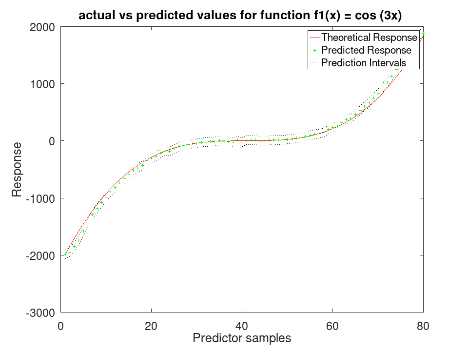
Plot the results

 figure
 [sortedY, indY] = sort (Ytrue(test (C)));
 plot (sortedY, 'r-');
 xlim ([0, sum(test(C))]);
 hold on
 plot (ypred(indY), 'g+')
 plot (yInt(indY,1),'k:')
 plot (yInt(indY,2),'k:')
 xlabel ('Predictor samples');
 ylabel ('Response');
 title ('actual vs predicted values for function f1(x) = cos (3x) ');
 legend ({'Theoretical Response', 'Predicted Response', 'Prediction Intervals'});

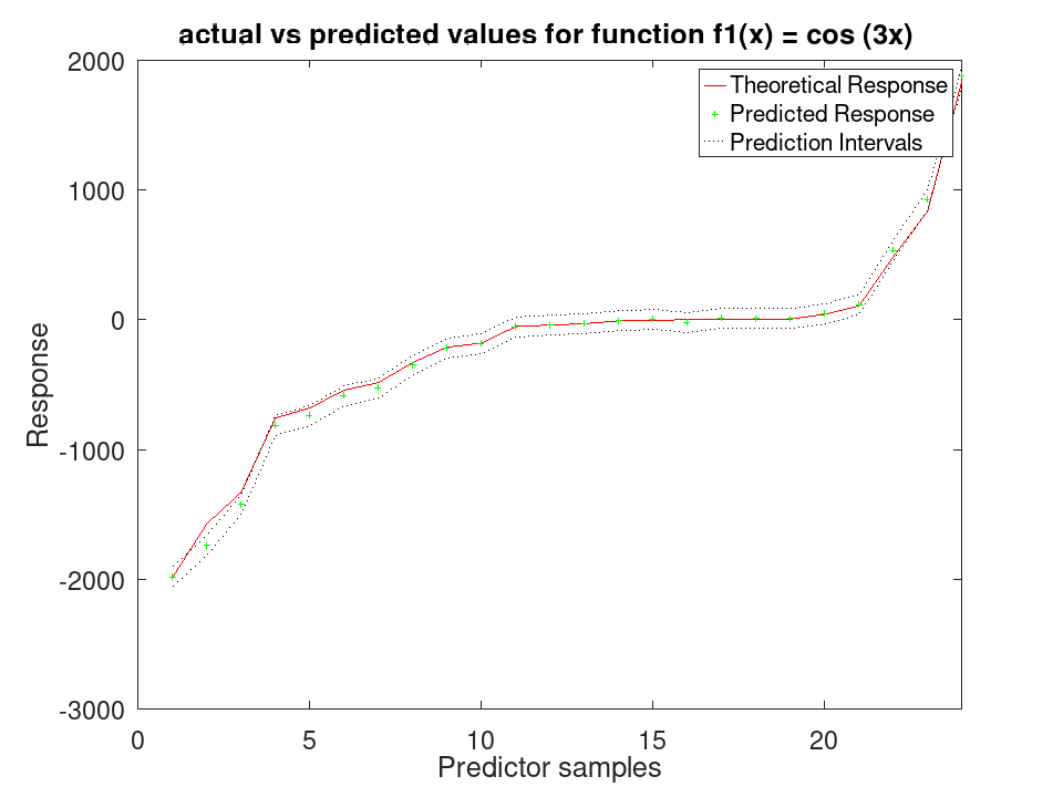
RegressionGAM: L = resubLoss (obj)

RegressionGAM: L = resubLoss (…, name, value)

L = resubLoss (obj) returns the weighted mean squared error of the model on the data it was fitted on. It accepts the same Name-Value pairs as loss.

See also: RegressionGAM, fitrgam, RegressionGAM.loss

Train a RegressionGAM Model for synthetic values

 rng (42);
 f1 = @(x) cos (3 * x);
 f2 = @(x) x .^ 3;
 x1 = 2 * rand (50, 1) - 1;
 x2 = 2 * rand (50, 1) - 1;
 y = f1(x1) + f2(x2);
 y = y + y .* 0.2 .* rand (50,1);
 X = [x1, x2];
 a = fitrgam (X, y)

a =

  RegressionGAM

             ResponseName: 'Y'
          NumObservations: 50
            NumPredictors: 2
        ResponseTransform: 'none'
                Intercept: 0.0671178
                    Knots: []
                    Order: []
                      Tol:

Declare two different functions

 rng (42);
 f1 = @(x) cos (3 * x);
 f2 = @(x) x .^ 3;

Generate 80 samples for f1 and f2

 x = [-4*pi:0.1*pi:4*pi-0.1*pi]';
 X1 = f1(x);
 X2 = f2(x);

Create a synthetic response by adding noise

 Ytrue = X1 + X2;
 Y = Ytrue + Ytrue .* 0.2 .* rand (80,1);

Assemble predictor data

 X = [X1, X2];

Train the GAM and test on the same data A standard deviation and a prediction interval come from the spline engine, which fits one; the boosted-tree engine reports none.

 a = fitrgam (X, Y, 'FitMethod', 'splines', 'order', [5, 5]);
 [ypred, ySDsd, yInt] = predict (a, X);

Plot the results

 figure
 [sortedY, indY] = sort (Ytrue);
 plot (sortedY, 'r-');
 xlim ([0, 80]);
 hold on
 plot (ypred(indY), 'g+')
 plot (yInt(indY,1), 'k:')
 plot (yInt(indY,2), 'k:')
 xlabel ('Predictor samples');
 ylabel ('Response');
 title ('actual vs predicted values for function f1(x) = cos (3x) ');
 legend ({'Theoretical Response', 'Predicted Response', 'Prediction Intervals'});

Use 30% Holdout partitioning for training and testing data

 C = cvpartition (80, 'HoldOut', 0.3);
 [ypred, ySDsd, yInt] = predict (a, X(test (C),:));

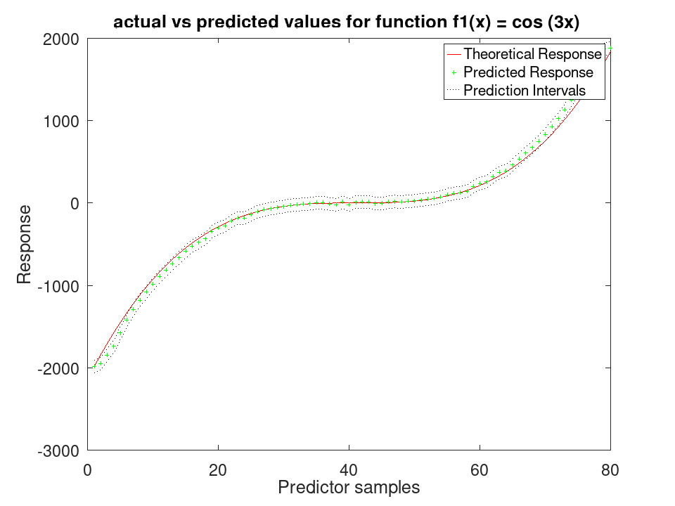
Plot the results

 figure
 [sortedY, indY] = sort (Ytrue(test (C)));
 plot (sortedY, 'r-');
 xlim ([0, sum(test(C))]);
 hold on
 plot (ypred(indY), 'g+')
 plot (yInt(indY,1),'k:')
 plot (yInt(indY,2),'k:')
 xlabel ('Predictor samples');
 ylabel ('Response');
 title ('actual vs predicted values for function f1(x) = cos (3x) ');
 legend ({'Theoretical Response', 'Predicted Response', 'Prediction Intervals'});

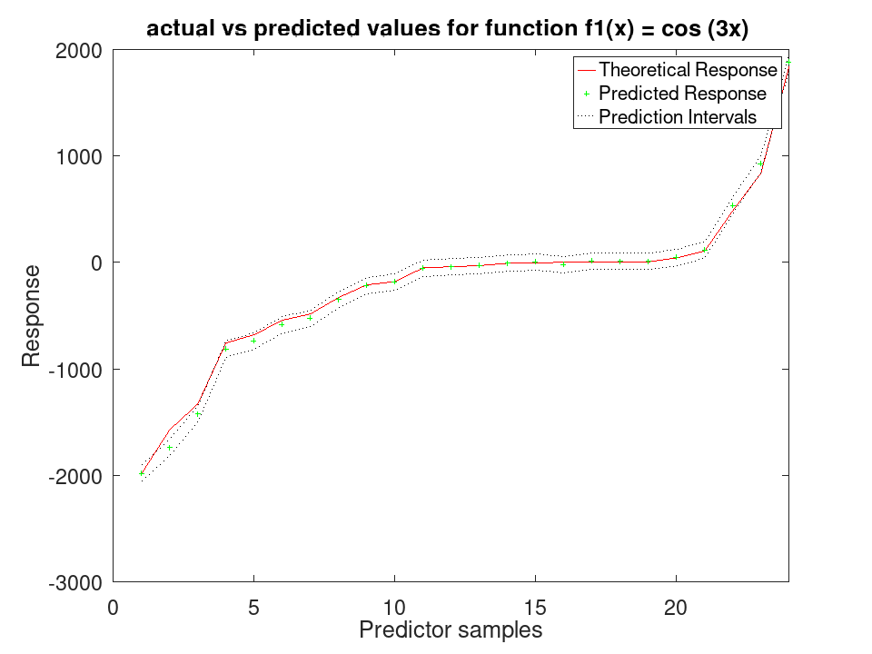
RegressionGAM: CVMdl = crossval (obj)

RegressionGAM: CVMdl = crossval (…, name, value)

CVMdl = crossval (obj) returns a cross-validated model object, CVMdl, from a trained model, obj, using 10-fold cross-validation by default.

CVMdl = crossval (obj, name, value) specifies additional name-value pair arguments to customize the cross-validation process.

`Name`	`Value`
`'KFold'`	Specify the number of folds to use in k-fold cross-validation. `"KFold", k`, where `k` is an integer greater than 1.
`'Holdout'`	Specify the fraction of the data to hold out for testing. `"Holdout", p`, where `p` is a scalar in the range (0,1).
`'Leaveout'`	Specify whether to perform leave-one-out cross-validation. `"Leaveout", Value`, where `Value` is ’on’ or ’off’.
`'CVPartition'`	Specify a `cvpartition` object used for cross-validation. `"CVPartition", cv`, where `isa (cv, "cvpartition")` = 1.

Train a RegressionGAM Model for synthetic values

 rng (42);
 f1 = @(x) cos (3 * x);
 f2 = @(x) x .^ 3;
 x1 = 2 * rand (50, 1) - 1;
 x2 = 2 * rand (50, 1) - 1;
 y = f1(x1) + f2(x2);
 y = y + y .* 0.2 .* rand (50,1);
 X = [x1, x2];
 a = fitrgam (X, y)

a =

  RegressionGAM

             ResponseName: 'Y'
          NumObservations: 50
            NumPredictors: 2
        ResponseTransform: 'none'
                Intercept: 0.0671178
                    Knots: []
                    Order: []
                      Tol:

Declare two different functions

 rng (42);
 f1 = @(x) cos (3 * x);
 f2 = @(x) x .^ 3;

Generate 80 samples for f1 and f2

 x = [-4*pi:0.1*pi:4*pi-0.1*pi]';
 X1 = f1(x);
 X2 = f2(x);

Create a synthetic response by adding noise

 Ytrue = X1 + X2;
 Y = Ytrue + Ytrue .* 0.2 .* rand (80,1);

Assemble predictor data

 X = [X1, X2];

Train the GAM and test on the same data A standard deviation and a prediction interval come from the spline engine, which fits one; the boosted-tree engine reports none.

 a = fitrgam (X, Y, 'FitMethod', 'splines', 'order', [5, 5]);
 [ypred, ySDsd, yInt] = predict (a, X);

Plot the results

 figure
 [sortedY, indY] = sort (Ytrue);
 plot (sortedY, 'r-');
 xlim ([0, 80]);
 hold on
 plot (ypred(indY), 'g+')
 plot (yInt(indY,1), 'k:')
 plot (yInt(indY,2), 'k:')
 xlabel ('Predictor samples');
 ylabel ('Response');
 title ('actual vs predicted values for function f1(x) = cos (3x) ');
 legend ({'Theoretical Response', 'Predicted Response', 'Prediction Intervals'});

Use 30% Holdout partitioning for training and testing data

 C = cvpartition (80, 'HoldOut', 0.3);
 [ypred, ySDsd, yInt] = predict (a, X(test (C),:));

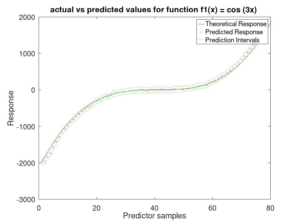
Plot the results

 figure
 [sortedY, indY] = sort (Ytrue(test (C)));
 plot (sortedY, 'r-');
 xlim ([0, sum(test(C))]);
 hold on
 plot (ypred(indY), 'g+')
 plot (yInt(indY,1),'k:')
 plot (yInt(indY,2),'k:')
 xlabel ('Predictor samples');
 ylabel ('Response');
 title ('actual vs predicted values for function f1(x) = cos (3x) ');
 legend ({'Theoretical Response', 'Predicted Response', 'Prediction Intervals'});

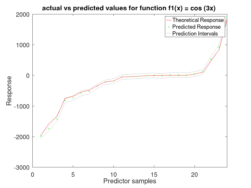
RegressionGAM: CMdl = compact (obj)

CMdl = compact (obj) returns a compact version of the model, which predicts as it does but keeps no training data.

See also: RegressionGAM, CompactRegressionGAM, fitrgam

Train a RegressionGAM Model for synthetic values

 rng (42);
 f1 = @(x) cos (3 * x);
 f2 = @(x) x .^ 3;
 x1 = 2 * rand (50, 1) - 1;
 x2 = 2 * rand (50, 1) - 1;
 y = f1(x1) + f2(x2);
 y = y + y .* 0.2 .* rand (50,1);
 X = [x1, x2];
 a = fitrgam (X, y)

a =

  RegressionGAM

             ResponseName: 'Y'
          NumObservations: 50
            NumPredictors: 2
        ResponseTransform: 'none'
                Intercept: 0.0671178
                    Knots: []
                    Order: []
                      Tol:

Declare two different functions

 rng (42);
 f1 = @(x) cos (3 * x);
 f2 = @(x) x .^ 3;

Generate 80 samples for f1 and f2

 x = [-4*pi:0.1*pi:4*pi-0.1*pi]';
 X1 = f1(x);
 X2 = f2(x);

Create a synthetic response by adding noise

 Ytrue = X1 + X2;
 Y = Ytrue + Ytrue .* 0.2 .* rand (80,1);

Assemble predictor data

 X = [X1, X2];

Train the GAM and test on the same data A standard deviation and a prediction interval come from the spline engine, which fits one; the boosted-tree engine reports none.

 a = fitrgam (X, Y, 'FitMethod', 'splines', 'order', [5, 5]);
 [ypred, ySDsd, yInt] = predict (a, X);

Plot the results

 figure
 [sortedY, indY] = sort (Ytrue);
 plot (sortedY, 'r-');
 xlim ([0, 80]);
 hold on
 plot (ypred(indY), 'g+')
 plot (yInt(indY,1), 'k:')
 plot (yInt(indY,2), 'k:')
 xlabel ('Predictor samples');
 ylabel ('Response');
 title ('actual vs predicted values for function f1(x) = cos (3x) ');
 legend ({'Theoretical Response', 'Predicted Response', 'Prediction Intervals'});

Use 30% Holdout partitioning for training and testing data

 C = cvpartition (80, 'HoldOut', 0.3);
 [ypred, ySDsd, yInt] = predict (a, X(test (C),:));

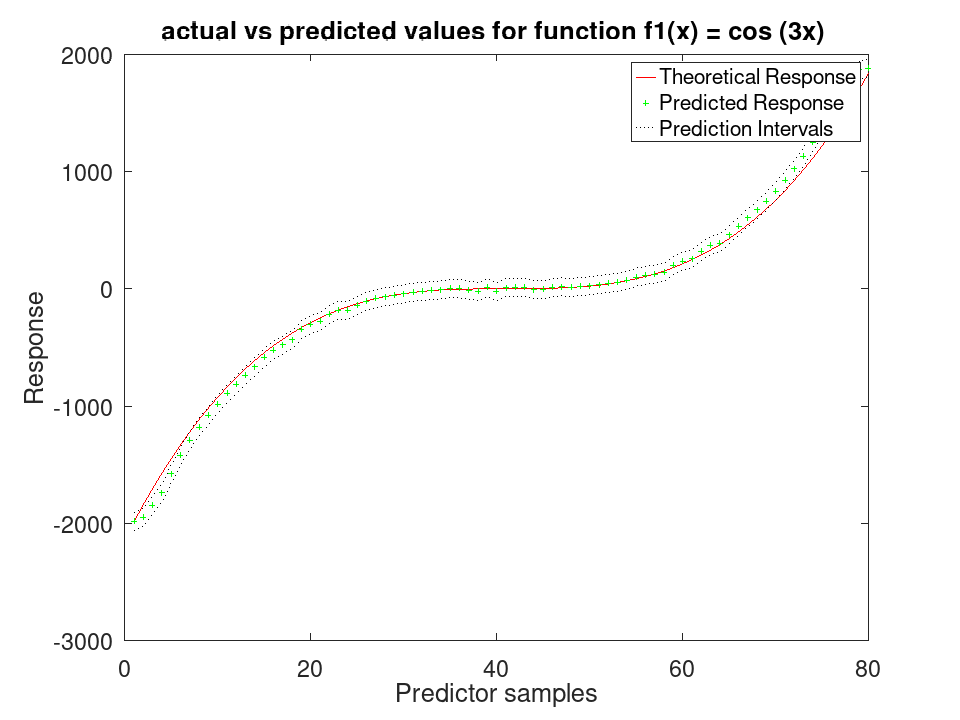
Plot the results

 figure
 [sortedY, indY] = sort (Ytrue(test (C)));
 plot (sortedY, 'r-');
 xlim ([0, sum(test(C))]);
 hold on
 plot (ypred(indY), 'g+')
 plot (yInt(indY,1),'k:')
 plot (yInt(indY,2),'k:')
 xlabel ('Predictor samples');
 ylabel ('Response');
 title ('actual vs predicted values for function f1(x) = cos (3x) ');
 legend ({'Theoretical Response', 'Predicted Response', 'Prediction Intervals'});

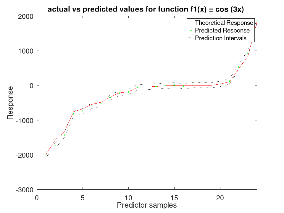
RegressionGAM: savemodel (obj, filename)

savemodel (obj, filename) saves a RegressionGAM object into a file defined by filename.

See also: loadmodel, fitrgam, RegressionGAM

Train a RegressionGAM Model for synthetic values

 rng (42);
 f1 = @(x) cos (3 * x);
 f2 = @(x) x .^ 3;
 x1 = 2 * rand (50, 1) - 1;
 x2 = 2 * rand (50, 1) - 1;
 y = f1(x1) + f2(x2);
 y = y + y .* 0.2 .* rand (50,1);
 X = [x1, x2];
 a = fitrgam (X, y)

a =

  RegressionGAM

             ResponseName: 'Y'
          NumObservations: 50
            NumPredictors: 2
        ResponseTransform: 'none'
                Intercept: 0.0671178
                    Knots: []
                    Order: []
                      Tol:

Declare two different functions

 rng (42);
 f1 = @(x) cos (3 * x);
 f2 = @(x) x .^ 3;

Generate 80 samples for f1 and f2

 x = [-4*pi:0.1*pi:4*pi-0.1*pi]';
 X1 = f1(x);
 X2 = f2(x);

Create a synthetic response by adding noise

 Ytrue = X1 + X2;
 Y = Ytrue + Ytrue .* 0.2 .* rand (80,1);

Assemble predictor data

 X = [X1, X2];

Train the GAM and test on the same data A standard deviation and a prediction interval come from the spline engine, which fits one; the boosted-tree engine reports none.

 a = fitrgam (X, Y, 'FitMethod', 'splines', 'order', [5, 5]);
 [ypred, ySDsd, yInt] = predict (a, X);

Plot the results

 figure
 [sortedY, indY] = sort (Ytrue);
 plot (sortedY, 'r-');
 xlim ([0, 80]);
 hold on
 plot (ypred(indY), 'g+')
 plot (yInt(indY,1), 'k:')
 plot (yInt(indY,2), 'k:')
 xlabel ('Predictor samples');
 ylabel ('Response');
 title ('actual vs predicted values for function f1(x) = cos (3x) ');
 legend ({'Theoretical Response', 'Predicted Response', 'Prediction Intervals'});

Use 30% Holdout partitioning for training and testing data

 C = cvpartition (80, 'HoldOut', 0.3);
 [ypred, ySDsd, yInt] = predict (a, X(test (C),:));

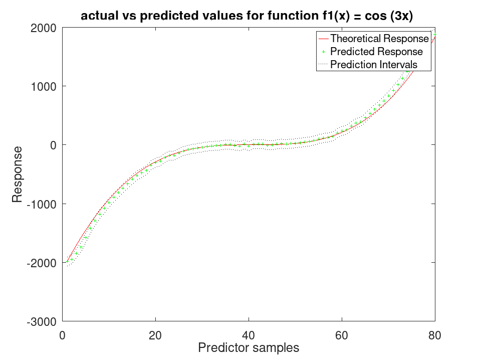
Plot the results

 figure
 [sortedY, indY] = sort (Ytrue(test (C)));
 plot (sortedY, 'r-');
 xlim ([0, sum(test(C))]);
 hold on
 plot (ypred(indY), 'g+')
 plot (yInt(indY,1),'k:')
 plot (yInt(indY,2),'k:')
 xlabel ('Predictor samples');
 ylabel ('Response');
 title ('actual vs predicted values for function f1(x) = cos (3x) ');
 legend ({'Theoretical Response', 'Predicted Response', 'Prediction Intervals'});

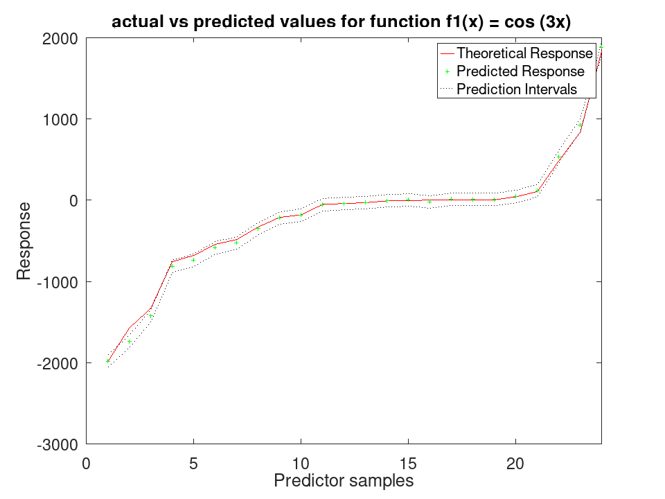
RegressionGAM: Mdl = resume (obj, numTrees)

Mdl = resume (obj, numTrees) adds numTrees more trees to obj and returns the result. The original model is not modified.

Training continues in the phase that ran last, which is what MATLAB does: a model carrying interaction terms gains interaction trees and its predictor shape functions are left alone, while a model without them gains predictor trees. A round starts at its initial learning rate whatever its number, so the model this returns is the model a single fit of the combined budget would have produced.

numTrees must be a positive integer scalar. Resuming raises where there is nothing left to gain, rather than returning the model unchanged, and it is not available under 'FitMethod', 'splines': a backfit that has converged to its tolerance has no budget to extend.

Train a RegressionGAM Model for synthetic values

 rng (42);
 f1 = @(x) cos (3 * x);
 f2 = @(x) x .^ 3;
 x1 = 2 * rand (50, 1) - 1;
 x2 = 2 * rand (50, 1) - 1;
 y = f1(x1) + f2(x2);
 y = y + y .* 0.2 .* rand (50,1);
 X = [x1, x2];
 a = fitrgam (X, y)

a =

  RegressionGAM

             ResponseName: 'Y'
          NumObservations: 50
            NumPredictors: 2
        ResponseTransform: 'none'
                Intercept: 0.0671178
                    Knots: []
                    Order: []
                      Tol:

Declare two different functions

 rng (42);
 f1 = @(x) cos (3 * x);
 f2 = @(x) x .^ 3;

Generate 80 samples for f1 and f2

 x = [-4*pi:0.1*pi:4*pi-0.1*pi]';
 X1 = f1(x);
 X2 = f2(x);

Create a synthetic response by adding noise

 Ytrue = X1 + X2;
 Y = Ytrue + Ytrue .* 0.2 .* rand (80,1);

Assemble predictor data

 X = [X1, X2];

Train the GAM and test on the same data A standard deviation and a prediction interval come from the spline engine, which fits one; the boosted-tree engine reports none.

 a = fitrgam (X, Y, 'FitMethod', 'splines', 'order', [5, 5]);
 [ypred, ySDsd, yInt] = predict (a, X);

Plot the results

 figure
 [sortedY, indY] = sort (Ytrue);
 plot (sortedY, 'r-');
 xlim ([0, 80]);
 hold on
 plot (ypred(indY), 'g+')
 plot (yInt(indY,1), 'k:')
 plot (yInt(indY,2), 'k:')
 xlabel ('Predictor samples');
 ylabel ('Response');
 title ('actual vs predicted values for function f1(x) = cos (3x) ');
 legend ({'Theoretical Response', 'Predicted Response', 'Prediction Intervals'});

Use 30% Holdout partitioning for training and testing data

 C = cvpartition (80, 'HoldOut', 0.3);
 [ypred, ySDsd, yInt] = predict (a, X(test (C),:));

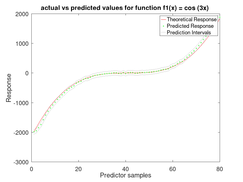
Plot the results

 figure
 [sortedY, indY] = sort (Ytrue(test (C)));
 plot (sortedY, 'r-');
 xlim ([0, sum(test(C))]);
 hold on
 plot (ypred(indY), 'g+')
 plot (yInt(indY,1),'k:')
 plot (yInt(indY,2),'k:')
 xlabel ('Predictor samples');
 ylabel ('Response');
 title ('actual vs predicted values for function f1(x) = cos (3x) ');
 legend ({'Theoretical Response', 'Predicted Response', 'Prediction Intervals'});

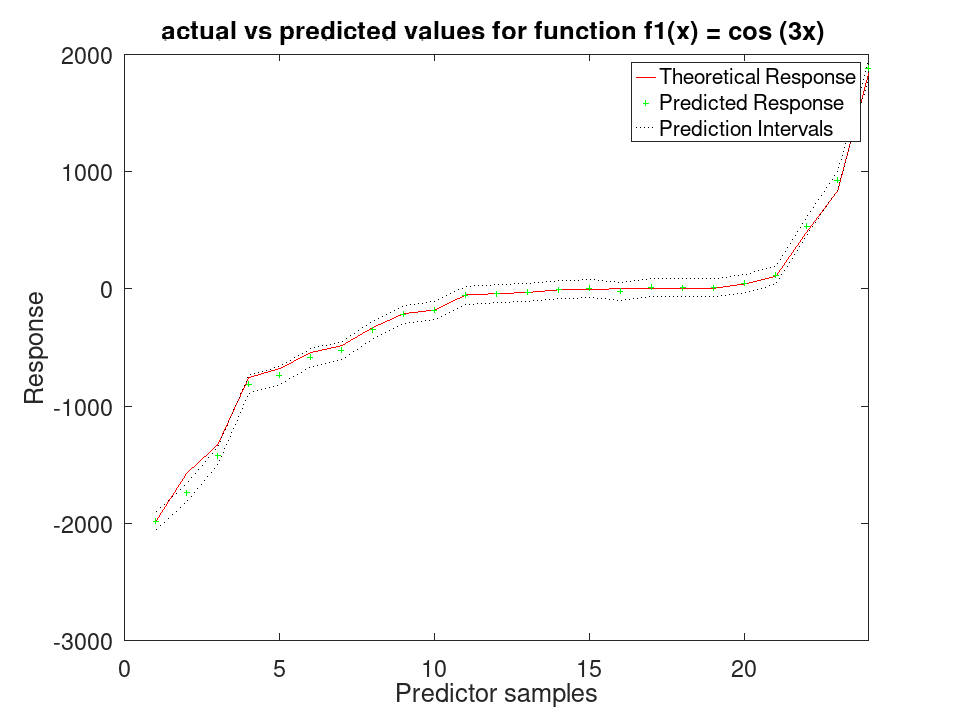
Examples

 rng (42);
 f1 = @(x) cos (3 * x);
 f2 = @(x) x .^ 3;
 x1 = 2 * rand (50, 1) - 1;
 x2 = 2 * rand (50, 1) - 1;
 y = f1(x1) + f2(x2);
 y = y + y .* 0.2 .* rand (50,1);
 X = [x1, x2];
 a = fitrgam (X, y)

a =

  RegressionGAM

             ResponseName: 'Y'
          NumObservations: 50
            NumPredictors: 2
        ResponseTransform: 'none'
                Intercept: 0.0671178
                    Knots: []
                    Order: []
                      Tol:

 rng (42);
 f1 = @(x) cos (3 * x);
 f2 = @(x) x .^ 3;

Generate 80 samples for f1 and f2

 x = [-4*pi:0.1*pi:4*pi-0.1*pi]';
 X1 = f1(x);
 X2 = f2(x);

Create a synthetic response by adding noise

 Ytrue = X1 + X2;
 Y = Ytrue + Ytrue .* 0.2 .* rand (80,1);

Assemble predictor data

 X = [X1, X2];

Train the GAM and test on the same data A standard deviation and a prediction interval come from the spline engine, which fits one; the boosted-tree engine reports none.

 a = fitrgam (X, Y, 'FitMethod', 'splines', 'order', [5, 5]);
 [ypred, ySDsd, yInt] = predict (a, X);

Plot the results

 figure
 [sortedY, indY] = sort (Ytrue);
 plot (sortedY, 'r-');
 xlim ([0, 80]);
 hold on
 plot (ypred(indY), 'g+')
 plot (yInt(indY,1), 'k:')
 plot (yInt(indY,2), 'k:')
 xlabel ('Predictor samples');
 ylabel ('Response');
 title ('actual vs predicted values for function f1(x) = cos (3x) ');
 legend ({'Theoretical Response', 'Predicted Response', 'Prediction Intervals'});

Use 30% Holdout partitioning for training and testing data

 C = cvpartition (80, 'HoldOut', 0.3);
 [ypred, ySDsd, yInt] = predict (a, X(test (C),:));

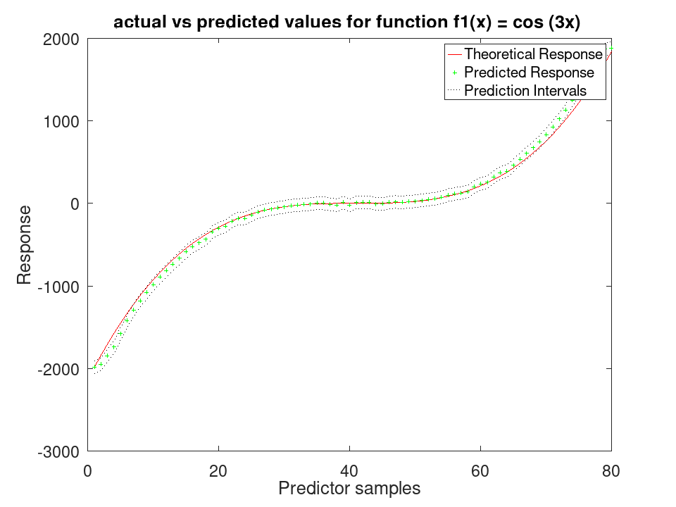
Plot the results

 figure
 [sortedY, indY] = sort (Ytrue(test (C)));
 plot (sortedY, 'r-');
 xlim ([0, sum(test(C))]);
 hold on
 plot (ypred(indY), 'g+')
 plot (yInt(indY,1),'k:')
 plot (yInt(indY,2),'k:')
 xlabel ('Predictor samples');
 ylabel ('Response');
 title ('actual vs predicted values for function f1(x) = cos (3x) ');
 legend ({'Theoretical Response', 'Predicted Response', 'Prediction Intervals'});

Categories &

Functions List

Descriptive Statistics

Descriptive Statistics

Data Manipulation

Data Manipulation

Hypothesis Testing

Hypothesis Testing

Experimental Design

Experimental Design

Regression

Regression

Machine Learning

Machine Learning

Clustering

Clustering

Nearest Neighbors

Nearest Neighbors

Anomaly Detection

Anomaly Detection

Dimensionality Reduction

Dimensionality Reduction

Model Evaluation

Model Evaluation

Markov Models

Markov Models

Random Sampling

Random Sampling

Distribution Classes

Distribution Classes

Distribution Fitting

Distribution Fitting

Distribution Functions

Distribution Functions

Distribution Statistics

Distribution Statistics

Distribution Wrappers

Distribution Wrappers

Plotting

Plotting

I/O

I/O

Utilities

Utilities

Class Definition: RegressionGAM

X

Y

NumObservations

RowsUsed

NumPredictors

PredictorNames

ResponseName

CategoricalPredictors

ExpandedPredictorNames

W

Intercept

Formula

Interactions

Knots

Order

DoF

Tol

IsStandardDeviationFit

BaseModel

ModelwInt

IntMatrix

BinEdges

PairDetectionBinEdges

ModelParameters

ReasonForTermination

FitMethod

TreeModel

HyperparameterOptimizationResults

ResponseTransform

RegressionGAM

addInteractions

predict

loss

resubPredict

resubLoss

Class Definition: `RegressionGAM`

`X`

`Y`

`NumObservations`

`RowsUsed`

`NumPredictors`

`PredictorNames`

`ResponseName`

`CategoricalPredictors`

`ExpandedPredictorNames`

`W`

`Intercept`

`Formula`

`Interactions`

`Knots`

`Order`

`DoF`

`Tol`

`IsStandardDeviationFit`

`BaseModel`

`ModelwInt`

`IntMatrix`

`BinEdges`

`PairDetectionBinEdges`

`ModelParameters`

`ReasonForTermination`

`FitMethod`

`TreeModel`

`HyperparameterOptimizationResults`

`ResponseTransform`

`RegressionGAM`

`addInteractions`

`predict`

`loss`

`resubPredict`

`resubLoss`

`crossval`

`compact`

`savemodel`

`resume`