Categories &
Functions List
- BetaDistribution
- BinomialDistribution
- BirnbaumSaundersDistribution
- BurrDistribution
- ExponentialDistribution
- ExtremeValueDistribution
- GammaDistribution
- GeneralizedExtremeValueDistribution
- GeneralizedParetoDistribution
- HalfNormalDistribution
- InverseGaussianDistribution
- LogisticDistribution
- LoglogisticDistribution
- LognormalDistribution
- LoguniformDistribution
- MultinomialDistribution
- NakagamiDistribution
- NegativeBinomialDistribution
- NormalDistribution
- PiecewiseLinearDistribution
- PoissonDistribution
- RayleighDistribution
- RicianDistribution
- tLocationScaleDistribution
- TriangularDistribution
- UniformDistribution
- WeibullDistribution
- betafit
- betalike
- binofit
- binolike
- bisafit
- bisalike
- burrfit
- burrlike
- evfit
- evlike
- expfit
- explike
- gamfit
- gamlike
- geofit
- gevfit_lmom
- gevfit
- gevlike
- gpfit
- gplike
- gumbelfit
- gumbellike
- hnfit
- hnlike
- invgfit
- invglike
- logifit
- logilike
- loglfit
- logllike
- lognfit
- lognlike
- nakafit
- nakalike
- nbinfit
- nbinlike
- normfit
- normlike
- poissfit
- poisslike
- raylfit
- rayllike
- ricefit
- ricelike
- tlsfit
- tlslike
- unidfit
- unifit
- wblfit
- wbllike
- betacdf
- betainv
- betapdf
- betarnd
- binocdf
- binoinv
- binopdf
- binornd
- bisacdf
- bisainv
- bisapdf
- bisarnd
- burrcdf
- burrinv
- burrpdf
- burrrnd
- bvncdf
- bvtcdf
- cauchycdf
- cauchyinv
- cauchypdf
- cauchyrnd
- chi2cdf
- chi2inv
- chi2pdf
- chi2rnd
- copulacdf
- copulapdf
- copularnd
- evcdf
- evinv
- evpdf
- evrnd
- expcdf
- expinv
- exppdf
- exprnd
- fcdf
- finv
- fpdf
- frnd
- gamcdf
- gaminv
- gampdf
- gamrnd
- geocdf
- geoinv
- geopdf
- geornd
- gevcdf
- gevinv
- gevpdf
- gevrnd
- gpcdf
- gpinv
- gppdf
- gprnd
- gumbelcdf
- gumbelinv
- gumbelpdf
- gumbelrnd
- hncdf
- hninv
- hnpdf
- hnrnd
- hygecdf
- hygeinv
- hygepdf
- hygernd
- invgcdf
- invginv
- invgpdf
- invgrnd
- iwishpdf
- iwishrnd
- jsucdf
- jsupdf
- laplacecdf
- laplaceinv
- laplacepdf
- laplacernd
- logicdf
- logiinv
- logipdf
- logirnd
- loglcdf
- loglinv
- loglpdf
- loglrnd
- logncdf
- logninv
- lognpdf
- lognrnd
- mnpdf
- mnrnd
- mvncdf
- mvnpdf
- mvnrnd
- mvtcdf
- mvtpdf
- mvtrnd
- mvtcdfqmc
- nakacdf
- nakainv
- nakapdf
- nakarnd
- nbincdf
- nbininv
- nbinpdf
- nbinrnd
- ncfcdf
- ncfinv
- ncfpdf
- ncfrnd
- nctcdf
- nctinv
- nctpdf
- nctrnd
- ncx2cdf
- ncx2inv
- ncx2pdf
- ncx2rnd
- normcdf
- norminv
- normpdf
- normrnd
- plcdf
- plinv
- plpdf
- plrnd
- poisscdf
- poissinv
- poisspdf
- poissrnd
- raylcdf
- raylinv
- raylpdf
- raylrnd
- ricecdf
- riceinv
- ricepdf
- ricernd
- tcdf
- tinv
- tpdf
- trnd
- tlscdf
- tlsinv
- tlspdf
- tlsrnd
- tricdf
- triinv
- tripdf
- trirnd
- unidcdf
- unidinv
- unidpdf
- unidrnd
- unifcdf
- unifinv
- unifpdf
- unifrnd
- vmcdf
- vminv
- vmpdf
- vmrnd
- wblcdf
- wblinv
- wblpdf
- wblrnd
- wienrnd
- wishpdf
- wishrnd
- adtest
- anova
- anova1
- anova2
- anovan
- bartlett_test
- barttest
- binotest
- chi2gof
- chi2test
- correlation_test
- fishertest
- friedman
- hotelling_t2test
- hotelling_t2test2
- kruskalwallis
- kstest
- kstest2
- levene_test
- manova1
- mcnemar_test
- multcompare
- ranksum
- regression_ftest
- regression_ttest
- runstest
- sampsizepwr
- signrank
- signtest
- tiedrank
- ttest
- ttest2
- vartest
- vartest2
- vartestn
- ztest
- ztest2
Function Reference: ridge
statistics: b = ridge (y, X, k)
statistics: b = ridge (y, X, k, scaled)
Ridge regression.
b = ridge (y, X, k) returns the vector of
coefficient estimates by applying ridge regression from the predictor matrix
X to the response vector y. Each value of b is the
coefficient for the respective ridge parameter given k. By default,
b is calculated after centering and scaling the predictors to have a
zero mean and standard deviation 1.
b = ridge (y, X, k, scaled) performs the
regression with the specified scaling of the coefficient estimates b.
When scaled = 0, the function restores the coefficients to the
scale of the original data thus is more useful for making predictions. When
scaled = 1, the coefficient estimates correspond to the scaled
centered data.
-
ymust be an numeric vector with the response data. -
Xmust be an numeric matrix with the predictor data. -
kmust be a numeric vector with the ridge parameters. -
scaledmust be a numeric scalar indicating whether the coefficient estimates in b are restored to the scale of the original data. By default,scaled = 1.
Further information about Ridge regression can be found at https://en.wikipedia.org/wiki/Ridge_regression
See also: lasso, stepwisefit, regress
Source Code: ridge
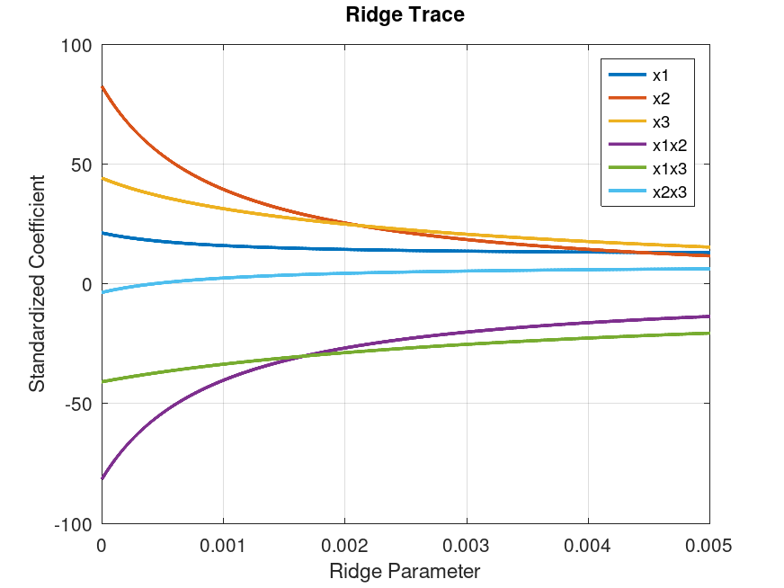
Example: 1
Perform ridge regression for a range of ridge parameters and observe how the coefficient estimates change based on the acetylene dataset.
 load acetylene
 X = [x1, x2, x3];
 x1x2 = x1 .* x2;
 x1x3 = x1 .* x3;
 x2x3 = x2 .* x3;
 D = [x1, x2, x3, x1x2, x1x3, x2x3];
 k = 0:1e-5:5e-3;
 b = ridge (y, D, k);
 figure
 plot (k, b, 'LineWidth', 2)
 ylim ([-100, 100])
 grid on
 xlabel ('Ridge Parameter')
 ylabel ('Standardized Coefficient')
 title ('Ridge Trace')
 legend ('x1', 'x2', 'x3', 'x1x2', 'x1x3', 'x2x3')
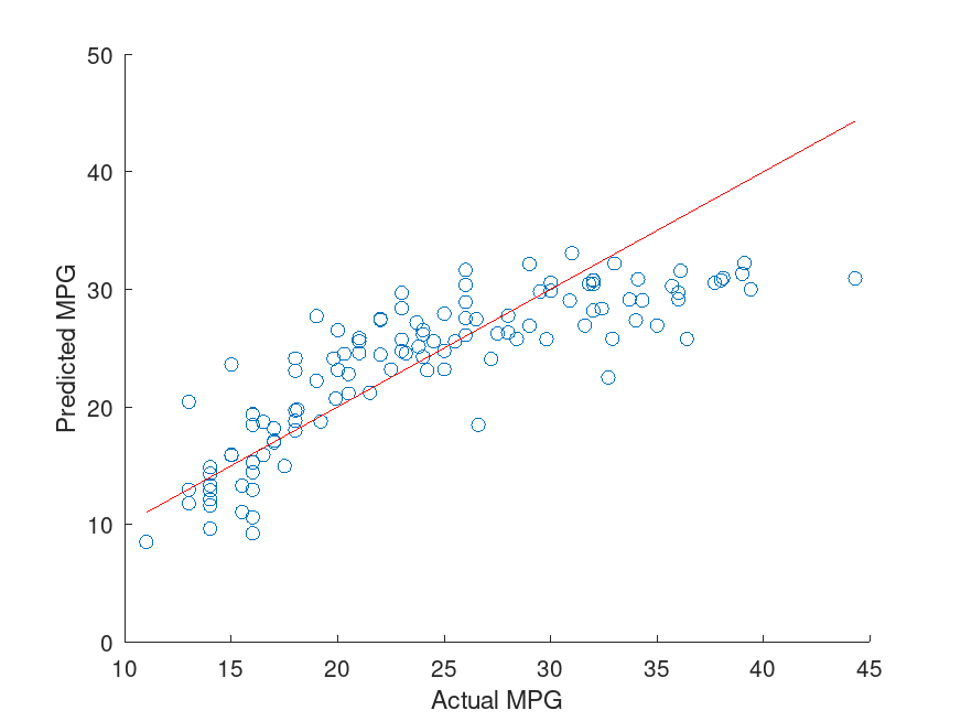
Example: 2
 load carbig
 X = [Acceleration Weight Displacement Horsepower];
 y = MPG;
 n = length (y);
 rand ('seed',1); % For reproducibility
 c = cvpartition (n,'HoldOut',0.3);
 idxTrain = training(c,1);
 idxTest = ! idxTrain;
 idxTrain = training(c,1);
 idxTest = ! idxTrain;
 k = 5;
 b = ridge (y(idxTrain),X(idxTrain,:),k,0);
Predict MPG values for the test data using the model.
 yhat = b(1) + X(idxTest,:)*b(2:end);
 scatter (y(idxTest),yhat)
 hold on
 plot (y(idxTest),y(idxTest),'r')
 xlabel ('Actual MPG')
 ylabel ('Predicted MPG')
 hold off