Categories &
Functions List
- BetaDistribution
- BinomialDistribution
- BirnbaumSaundersDistribution
- BurrDistribution
- ExponentialDistribution
- ExtremeValueDistribution
- GammaDistribution
- GeneralizedExtremeValueDistribution
- GeneralizedParetoDistribution
- HalfNormalDistribution
- InverseGaussianDistribution
- LogisticDistribution
- LoglogisticDistribution
- LognormalDistribution
- LoguniformDistribution
- MultinomialDistribution
- NakagamiDistribution
- NegativeBinomialDistribution
- NormalDistribution
- PiecewiseLinearDistribution
- PoissonDistribution
- RayleighDistribution
- RicianDistribution
- tLocationScaleDistribution
- TriangularDistribution
- UniformDistribution
- WeibullDistribution
- betafit
- betalike
- binofit
- binolike
- bisafit
- bisalike
- burrfit
- burrlike
- evfit
- evlike
- expfit
- explike
- gamfit
- gamlike
- geofit
- gevfit_lmom
- gevfit
- gevlike
- gpfit
- gplike
- gumbelfit
- gumbellike
- hnfit
- hnlike
- invgfit
- invglike
- logifit
- logilike
- loglfit
- logllike
- lognfit
- lognlike
- nakafit
- nakalike
- nbinfit
- nbinlike
- normfit
- normlike
- poissfit
- poisslike
- raylfit
- rayllike
- ricefit
- ricelike
- tlsfit
- tlslike
- unidfit
- unifit
- wblfit
- wbllike
- betacdf
- betainv
- betapdf
- betarnd
- binocdf
- binoinv
- binopdf
- binornd
- bisacdf
- bisainv
- bisapdf
- bisarnd
- burrcdf
- burrinv
- burrpdf
- burrrnd
- bvncdf
- bvtcdf
- cauchycdf
- cauchyinv
- cauchypdf
- cauchyrnd
- chi2cdf
- chi2inv
- chi2pdf
- chi2rnd
- copulacdf
- copulapdf
- copularnd
- evcdf
- evinv
- evpdf
- evrnd
- expcdf
- expinv
- exppdf
- exprnd
- fcdf
- finv
- fpdf
- frnd
- gamcdf
- gaminv
- gampdf
- gamrnd
- geocdf
- geoinv
- geopdf
- geornd
- gevcdf
- gevinv
- gevpdf
- gevrnd
- gpcdf
- gpinv
- gppdf
- gprnd
- gumbelcdf
- gumbelinv
- gumbelpdf
- gumbelrnd
- hncdf
- hninv
- hnpdf
- hnrnd
- hygecdf
- hygeinv
- hygepdf
- hygernd
- invgcdf
- invginv
- invgpdf
- invgrnd
- iwishpdf
- iwishrnd
- jsucdf
- jsupdf
- laplacecdf
- laplaceinv
- laplacepdf
- laplacernd
- logicdf
- logiinv
- logipdf
- logirnd
- loglcdf
- loglinv
- loglpdf
- loglrnd
- logncdf
- logninv
- lognpdf
- lognrnd
- mnpdf
- mnrnd
- mvncdf
- mvnpdf
- mvnrnd
- mvtcdf
- mvtpdf
- mvtrnd
- mvtcdfqmc
- nakacdf
- nakainv
- nakapdf
- nakarnd
- nbincdf
- nbininv
- nbinpdf
- nbinrnd
- ncfcdf
- ncfinv
- ncfpdf
- ncfrnd
- nctcdf
- nctinv
- nctpdf
- nctrnd
- ncx2cdf
- ncx2inv
- ncx2pdf
- ncx2rnd
- normcdf
- norminv
- normpdf
- normrnd
- plcdf
- plinv
- plpdf
- plrnd
- poisscdf
- poissinv
- poisspdf
- poissrnd
- raylcdf
- raylinv
- raylpdf
- raylrnd
- ricecdf
- riceinv
- ricepdf
- ricernd
- tcdf
- tinv
- tpdf
- trnd
- tlscdf
- tlsinv
- tlspdf
- tlsrnd
- tricdf
- triinv
- tripdf
- trirnd
- unidcdf
- unidinv
- unidpdf
- unidrnd
- unifcdf
- unifinv
- unifpdf
- unifrnd
- vmcdf
- vminv
- vmpdf
- vmrnd
- wblcdf
- wblinv
- wblpdf
- wblrnd
- wienrnd
- wishpdf
- wishrnd
- adtest
- anova
- anova1
- anova2
- anovan
- bartlett_test
- barttest
- binotest
- chi2gof
- chi2test
- correlation_test
- fishertest
- friedman
- hotelling_t2test
- hotelling_t2test2
- kruskalwallis
- kstest
- kstest2
- levene_test
- manova1
- mcnemar_test
- multcompare
- ranksum
- regression_ftest
- regression_ttest
- runstest
- sampsizepwr
- signrank
- signtest
- tiedrank
- ttest
- ttest2
- vartest
- vartest2
- vartestn
- ztest
- ztest2
Class Definition: BurrDistribution
statistics: BurrDistribution
Burr probability distribution object.
A BurrDistribution object consists of parameters, a model
description, and sample data for a Burr probability distribution.
The Burr distribution is a continuous probability distribution that models a non-negative random variable, commonly used to model household income. It is defined by a scale parameter alpha and two shape parameters c and k.
There are several ways to create a BurrDistribution object.
- Fit a distribution to data using the
fitdistfunction. - Create a distribution with fixed parameter values using the
makedistfunction. - Use the constructor
BurrDistribution (alpha, c,
 k)
to create a Burr distribution with fixed parameter values alpha, c, and k. - Use the static method
BurrDistribution.fit (x,
 alpha, censor, freq, options)
to fit a distribution to the data in x using the same input arguments as theburrfitfunction.
It is highly recommended to use fitdist and makedist
functions to create probability distribution objects, instead of the class
constructor or the aforementioned static method.
Further information about the Burr distribution can be found at https://en.wikipedia.org/wiki/Burr_distribution
See also: fitdist, makedist, burrcdf, burrinv, burrpdf, burrrnd, burrfit, burrlike, burrstat
Source Code: BurrDistribution
The BurrDistribution class contains the following properties:
A positive scalar value characterizing the scale of the Burr
distribution. You can access the alpha property using dot name
assignment.
Example: 1
Create a Burr distribution with default parameters
pd = makedist ("Burr")
pd =
  BurrDistribution

  Burr distribution
    alpha = 1
        c = 1
        k = 1
Query parameter 'alpha' (scale parameter)
pd.alpha
ans = 1
Set parameter 'alpha'
pd.alpha = 2
pd =
  BurrDistribution

  Burr distribution
    alpha = 2
        c = 1
        k = 1
Use this to initialize or modify the scale parameter of a Burr distribution. The scale parameter must be a positive real scalar.
Example: 2
Create a Burr distribution object by calling its constructor
pd = BurrDistribution (1.5, 2, 1)
pd =
  BurrDistribution

  Burr distribution
    alpha = 1.5
        c =   2
        k =   1
Query parameter 'alpha'
pd.alpha
ans = 1.5000
This demonstrates direct construction with a specific scale parameter, ideal for modeling specific household income distributions.
A positive scalar value characterizing the first shape parameter of the
Burr distribution. You can access the c property using dot name
assignment.
Example: 1
Create a Burr distribution with default parameters
pd = makedist ("Burr")
pd =
  BurrDistribution

  Burr distribution
    alpha = 1
        c = 1
        k = 1
Query parameter 'c' (first shape parameter)
pd.c
ans = 1
Set parameter 'c'
pd.c = 3
pd =
  BurrDistribution

  Burr distribution
    alpha = 1
        c = 3
        k = 1
Use this to initialize or modify the first shape parameter in a Burr distribution. The first shape parameter must be a positive real scalar.
Example: 2
Create a Burr distribution object by calling its constructor
pd = BurrDistribution (1, 3, 1)
pd =
  BurrDistribution

  Burr distribution
    alpha = 1
        c = 3
        k = 1
Query parameter 'c'
pd.c
ans = 3
This shows how to set the first shape parameter directly via the constructor, useful for modeling variability in non-negative data like household income.
A positive scalar value characterizing the second shape parameter of the
Burr distribution. You can access the k property using dot name
assignment.
Example: 1
Create a Burr distribution with default parameters
pd = makedist ("Burr")
pd =
  BurrDistribution

  Burr distribution
    alpha = 1
        c = 1
        k = 1
Query parameter 'k' (second shape parameter)
pd.k
ans = 1
Set parameter 'k'
pd.k = 2
pd =
  BurrDistribution

  Burr distribution
    alpha = 1
        c = 1
        k = 2
Use this to initialize or modify the second shape parameter in a Burr distribution. The second shape parameter must be a positive real scalar.
Example: 2
Create a Burr distribution object by calling its constructor
pd = BurrDistribution (1, 2, 2)
pd =
  BurrDistribution

  Burr distribution
    alpha = 1
        c = 2
        k = 2
Query parameter 'k'
pd.k
ans = 2
This shows how to set the second shape parameter directly via the constructor, ideal for tailoring the tail behavior in distributions for income data.
A character vector specifying the name of the probability distribution object. This property is read-only.
A scalar integer value specifying the number of parameters characterizing the probability distribution. This property is read-only.
A cell array of character vectors with each element containing the name of a distribution parameter. This property is read-only.
A cell array of character vectors with each element containing a short description of a distribution parameter. This property is read-only.
A numeric vector containing the values of the distribution
parameters. This property is read-only. You can change the distribution
parameters by assigning new values to the alpha, c, and
k properties.
A numeric matrix containing the variance-covariance of the parameter estimates. Diagonal elements contain the variance of each estimated parameter, and non-diagonal elements contain the covariance between the parameter estimates. The covariance matrix is only meaningful when the distribution was fitted to data. If the distribution object was created with fixed parameters, or a parameter of a fitted distribution is modified, then all elements of the variance-covariance are zero. This property is read-only.
A logical vector specifying which parameters are fixed and
which are estimated. true values correspond to fixed parameters,
false values correspond to parameter estimates. This property is
read-only.
A numeric vector specifying the truncation interval for the
probability distribution. First element contains the lower boundary,
second element contains the upper boundary. This property is read-only.
You can only truncate a probability distribution with the
truncate method.
A logical scalar value specifying whether a probability distribution is truncated or not. This property is read-only.
A scalar structure containing the following fields:
-
data: a numeric vector containing the data used for distribution fitting. -
cens: an empty array, sinceBurrDistributiondoes not allow censoring. -
freq: a numeric vector of non-negative integer values containing the frequency information corresponding to the elements of the data used for distribution fitting. If no frequency vector was used for distribution fitting, then this field defaults to an empty array.
The BurrDistribution class offers the following public methods:
BurrDistribution: p = cdf (pd, x)
BurrDistribution: p = cdf (pd, x,
'upper')
p = cdf (pd, x) computes the CDF of the
probability distribution object, pd, evaluated at the values in
x.
p = cdf (…, returns the complement of
the CDF of the probability distribution object, pd, evaluated at
the values in x.
'upper')
Example: 1
Plot various CDFs from the Burr distribution
 x = 0:0.01:5;
 pd1 = makedist ("Burr", "alpha", 1, "c", 2, "k", 1);
 pd2 = makedist ("Burr", "alpha", 1, "c", 3, "k", 1);
 pd3 = makedist ("Burr", "alpha", 1, "c", 4, "k", 1);
 p1 = cdf (pd1, x);
 p2 = cdf (pd2, x);
 p3 = cdf (pd3, x);
 plot (x, p1, "-b", x, p2, "-g", x, p3, "-r")
 grid on
 legend ({"alpha=1, c=2, k=1", "alpha=1, c=3, k=1", "alpha=1, c=4, k=1"}, ...
         "location", "southeast")
 title ("Burr CDF")
 xlabel ("values in x")
 ylabel ("Cumulative probability")
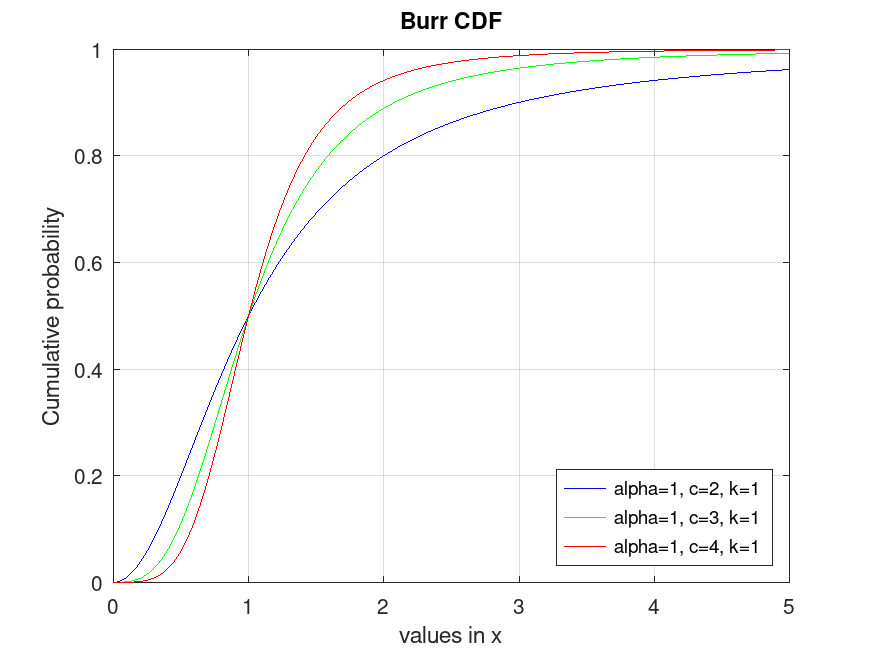
Use this to compute and visualize the cumulative distribution function for different Burr distributions, showing how probability accumulates over non-negative values like income levels.
BurrDistribution: x = icdf (pd, p)
x = icdf (pd, p) computes the quantile (the
inverse of the CDF) of the probability distribution object, pd,
evaluated at the values in p.
Example: 1
Plot various iCDFs from the Burr distribution
 p = 0.001:0.001:0.999;
 pd1 = makedist ("Burr", "alpha", 1, "c", 2, "k", 1);
 pd2 = makedist ("Burr", "alpha", 1, "c", 3, "k", 1);
 pd3 = makedist ("Burr", "alpha", 1, "c", 4, "k", 1);
 x1 = icdf (pd1, p);
 x2 = icdf (pd2, p);
 x3 = icdf (pd3, p);
 plot (p, x1, "-b", p, x2, "-g", p, x3, "-r")
 grid on
 legend ({"alpha=1, c=2, k=1", "alpha=1, c=3, k=1", "alpha=1, c=4, k=1"}, ...
         "location", "northwest")
 title ("Burr iCDF")
 xlabel ("Probability")
 ylabel ("values in x")
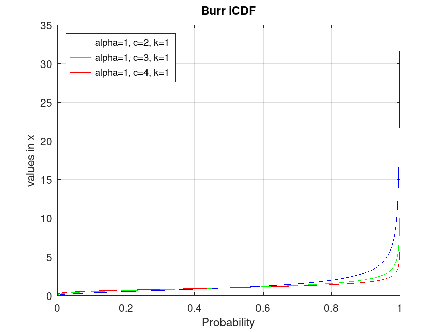
This demonstrates the inverse CDF (quantiles) for Burr distributions, useful for finding the value (e.g., income level) corresponding to given probabilities.
BurrDistribution: r = iqr (pd)
r = iqr (pd) computes the interquartile range of the
probability distribution object, pd.
Example: 1
Compute the interquartile range for a Burr distribution
pd = makedist ("Burr", "alpha", 1, "c", 2, "k", 1)
pd =
  BurrDistribution

  Burr distribution
    alpha = 1
        c = 2
        k = 1
iqr_value = iqr (pd)
iqr_value = 1.1547
Use this to calculate the interquartile range, which measures the spread of the middle 50% of the distribution, useful for understanding variability in data like household income.
BurrDistribution: m = mean (pd)
m = mean (pd) computes the mean of the probability
distribution object, pd.
Example: 1
Compute the mean for different Burr distributions
 pd1 = makedist ("Burr", "alpha", 1, "c", 2, "k", 1);
 pd2 = makedist ("Burr", "alpha", 1, "c", 3, "k", 1);
 mean1 = mean (pd1)
mean1 = 1.5708
mean2 = mean (pd2)
mean2 = 1.2092
This shows how to compute the expected value for Burr distributions with different shape parameters, provided the parameters allow a finite mean (e.g., when c * k > 1).
BurrDistribution: m = median (pd)
m = median (pd) computes the median of the probability
distribution object, pd.
Example: 1
Compute the median for different Burr distributions
 pd1 = makedist ("Burr", "alpha", 1, "c", 2, "k", 1);
 pd2 = makedist ("Burr", "alpha", 1, "c", 3, "k", 1);
 median1 = median (pd1)
median1 = 1
median2 = median (pd2)
median2 = 1
Use this to find the median value, which splits the distribution into two equal probability halves, e.g., median household income.
BurrDistribution: nlogL = negloglik (pd)
nlogL = negloglik (pd) computes the negative
loglikelihood of the probability distribution object, pd.
Example: 1
Compute the negative loglikelihood for a fitted Burr distribution
pd = makedist ("Burr", "alpha", 1, "c", 2, "k", 1)
pd =
  BurrDistribution

  Burr distribution
    alpha = 1
        c = 2
        k = 1
 rand ("seed", 21);
 data = random (pd, 100, 1);
 pd_fitted = fitdist (data, "Burr")
pd_fitted =
  BurrDistribution

  Burr distribution
    alpha = 1.18986   [1.01271, 1.39799]
        c = 1.91252   [1.62314, 2.25348]
        k = 1.30385   [0.625566, 2.71757]
nlogL = negloglik (pd_fitted)
nlogL = -123.35
This is useful for assessing the fit of a Burr distribution to data; lower values indicate a better fit, e.g., for income modeling.
BurrDistribution: ci = paramci (pd)
BurrDistribution: ci = paramci (pd, Name, Value)
ci = paramci (pd) computes the lower and upper
boundaries of the 95% confidence interval for each parameter of the
probability distribution object, pd.
ci = paramci (pd, Name, Value) computes
the
confidence intervals with additional options specified by
Name-Value pair arguments listed below.
| Name | Value | |
|---|---|---|
'Alpha' | A scalar value in the range specifying the significance level for the confidence interval. The default value 0.05 corresponds to a 95% confidence interval. | |
'Parameter' | A character vector or a cell array of
character vectors specifying the parameter names for which to compute
confidence intervals. By default, paramci computes confidence
intervals for all distribution parameters. |
paramci is meaningful only when pd is fitted to data,
otherwise an empty array, [], is returned.
Example: 1
Compute confidence intervals for parameters of a fitted Burr distribution
pd = makedist ("Burr", "alpha", 1, "c", 2, "k", 1)
pd =
  BurrDistribution

  Burr distribution
    alpha = 1
        c = 2
        k = 1
 rand ("seed", 21);
 data = random (pd, 1000, 1);
 pd_fitted = fitdist (data, "Burr")
pd_fitted =
  BurrDistribution

  Burr distribution
    alpha =  1.00315   [0.951509, 1.0576]
        c =  2.04261   [1.93888, 2.1519]
        k = 0.974629   [0.777103, 1.22236]
ci = paramci (pd_fitted, "Alpha", 0.05)
ci =

   0.9515   1.9389   0.7771
   1.0576   2.1519   1.2224
Use this to obtain confidence intervals for the estimated parameters (alpha, c, k), providing a range of plausible values given the data, e.g., for uncertainty in income distribution parameters.
BurrDistribution: y = pdf (pd, x)
y = pdf (pd, x) computes the PDF of the
probability distribution object, pd, evaluated at the values in
x.
Example: 1
Plot various PDFs from the Burr distribution
 x = 0:0.01:5;
 pd1 = makedist ("Burr", "alpha", 1, "c", 2, "k", 1);
 pd2 = makedist ("Burr", "alpha", 1, "c", 3, "k", 1);
 pd3 = makedist ("Burr", "alpha", 1, "c", 4, "k", 1);
 y1 = pdf (pd1, x);
 y2 = pdf (pd2, x);
 y3 = pdf (pd3, x);
 plot (x, y1, "-b", x, y2, "-g", x, y3, "-r")
 grid on
 legend ({"alpha=1, c=2, k=1", "alpha=1, c=3, k=1", "alpha=1, c=4, k=1"}, ...
         "location", "northeast")
 title ("Burr PDF")
 xlabel ("values in x")
 ylabel ("Probability density")
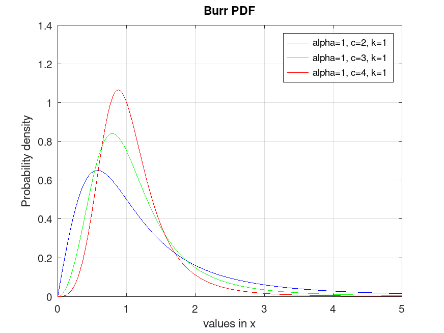
This visualizes the probability density function for Burr distributions, showing the likelihood of different values, e.g., income levels.
BurrDistribution: plot (pd)
BurrDistribution: plot (pd, Name, Value)
BurrDistribution: h = plot (…)
plot (pd) plots a probability density function (PDF) of the
probability distribution object pd. If pd contains data,
which have been fitted by fitdist, the PDF is superimposed over a
histogram of the data.
plot (pd, Name, Value) specifies additional
options with the Name-Value pair arguments listed below.
| Name | Value | |
|---|---|---|
'PlotType' | A character vector specifying the plot
type. 'pdf' plots the probability density function (PDF). When
pd is fit to data, the PDF is superimposed on a histogram of the
data. 'cdf' plots the cumulative density function (CDF). When
pd is fit to data, the CDF is superimposed over an empirical CDF.
'probability' plots a probability plot using a CDF of the data
and a CDF of the fitted probability distribution. This option is
available only when pd is fitted to data. | |
'Discrete' | A logical scalar to specify whether to
plot the PDF or CDF of a discrete distribution object as a line plot or a
stem plot, by specifying false or true, respectively. By
default, it is true for discrete distributions and false
for continuous distributions. When pd is a continuous distribution
object, option is ignored. | |
'Parent' | An axes graphics object for plot. If
not specified, the plot function plots into the current axes or
creates a new axes object if one does not exist. |
h = plot (…) returns a graphics handle to the plotted
objects.
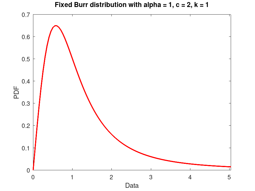
Example: 1
Create a Burr distribution with fixed parameters alpha = 1, c = 2, k = 1 and plot its PDF.
pd = makedist ("Burr", "alpha", 1, "c", 2, "k", 1)
pd =
  BurrDistribution

  Burr distribution
    alpha = 1
        c = 2
        k = 1
 plot (pd)
 title ("Fixed Burr distribution with alpha = 1, c = 2, k = 1")
Example: 2
Generate a data set of 100 random samples from a Burr distribution with parameters alpha = 1, c = 2, k = 1. Fit a Burr distribution to this data and plot its CDF superimposed over an empirical CDF.
pd_fixed = makedist ("Burr", "alpha", 1, "c", 2, "k", 1)
pd_fixed =
  BurrDistribution

  Burr distribution
    alpha = 1
        c = 2
        k = 1
 rand ("seed", 21);
 data = random (pd_fixed, 100, 1);
 pd_fitted = fitdist (data, "Burr")
pd_fitted =
  BurrDistribution

  Burr distribution
    alpha = 1.18986   [1.01271, 1.39799]
        c = 1.91252   [1.62314, 2.25348]
        k = 1.30385   [0.625566, 2.71757]
 plot (pd_fitted, "PlotType", "cdf")
 txt = "Fitted Burr distribution with alpha = %0.2f, c = %0.2f, k = %0.2f";
 title (sprintf (txt, pd_fitted.alpha, pd_fitted.c, pd_fitted.k))
 legend ({"empirical CDF", "fitted CDF"}, "location", "southeast")
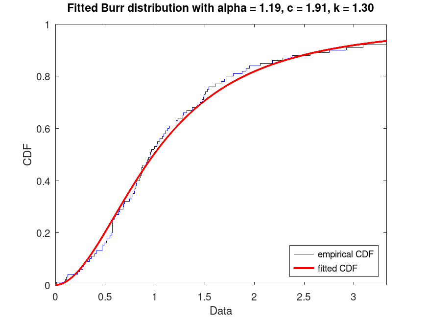
Use this to visualize the fitted CDF compared to the empirical CDF of the data, useful for assessing model fit in income data.
Example: 3
Generate a data set of 200 random samples from a Burr distribution with parameters alpha = 1, c = 2, k = 1. Display a probability plot for the Burr distribution fit to the data.
pd_fixed = makedist ("Burr", "alpha", 1, "c", 2, "k", 1)
pd_fixed =
  BurrDistribution

  Burr distribution
    alpha = 1
        c = 2
        k = 1
 rand ("seed", 21);
 data = random (pd_fixed, 200, 1);
 pd_fitted = fitdist (data, "Burr")
pd_fitted =
  BurrDistribution

  Burr distribution
    alpha = 1.23729   [1.10047, 1.39113]
        c = 1.88943   [1.68443, 2.11939]
        k = 1.27534   [0.720502, 2.25744]
 plot (pd_fitted, "PlotType", "probability")
 txt = strcat ("Probability plot of fitted Burr distribution with ", ...
               "alpha = %0.2f, c = %0.2f, k = %0.2f");
 title (sprintf (txt, pd_fitted.alpha, pd_fitted.c, pd_fitted.k))
 legend ({"empirical CDF", "fitted CDF"}, "location", "southeast")
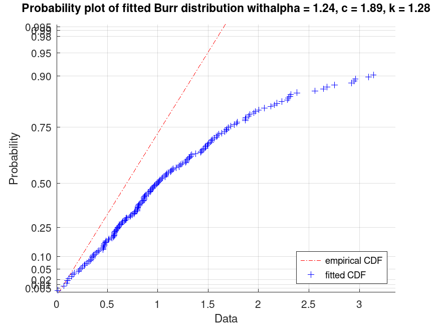
This creates a probability plot to compare the fitted distribution to the data, useful for checking if the Burr model is appropriate for the dataset.
BurrDistribution: [nlogL, param] = proflik (pd, pnum)
BurrDistribution: [nlogL, param] = proflik (pd, pnum,
'Display', display)BurrDistribution: [nlogL, param] = proflik (pd, pnum, setparam)
BurrDistribution: [nlogL, param] = proflik (pd, pnum, setparam,
'Display', display)
[nlogL, param] = proflik (pd, pnum)
returns a vector nlogL of negative loglikelihood values and a
vector param of corresponding parameter values for the parameter in
the position indicated by pnum. By default, proflik uses
the lower and upper bounds of the 95% confidence interval and computes
100 equispaced values for the selected parameter. pd must be
fitted to data.
[nlogL, param] = proflik (pd, pnum,
also plots the profile likelihood
against the default range of the selected parameter.
'Display', 'on')
[nlogL, param] = proflik (pd, pnum,
 setparam)
defines a user-defined range of the selected parameter.
[nlogL, param] = proflik (pd, pnum,
setparam, also plots the profile
likelihood against the user-defined range of the selected parameter.
'Display', 'on')
For the Burr distribution, pnum = 1 selects the parameter
alpha, pnum = 2 selects the parameter c,
and pnum = 3 selects the parameter k.
When opted to display the profile likelihood plot, proflik also
plots the baseline loglikelihood computed at the lower bound of the 95%
confidence interval and estimated maximum likelihood. The latter might
not be observable if it is outside of the used-defined range of parameter
values.
Example: 1
Compute and plot the profile likelihood for the first shape parameter of a fitted Burr distribution
pd = makedist ("Burr", "alpha", 1, "c", 2, "k", 1)
pd =
  BurrDistribution

  Burr distribution
    alpha = 1
        c = 2
        k = 1
 rand ("seed", 21);
 data = random (pd, 1000, 1);
 pd_fitted = fitdist (data, "Burr")
pd_fitted =
  BurrDistribution

  Burr distribution
    alpha =  1.00315   [0.951509, 1.0576]
        c =  2.04261   [1.93888, 2.1519]
        k = 0.974629   [0.777103, 1.22236]
[nlogL, param] = proflik (pd_fitted, 2, "Display", "on");
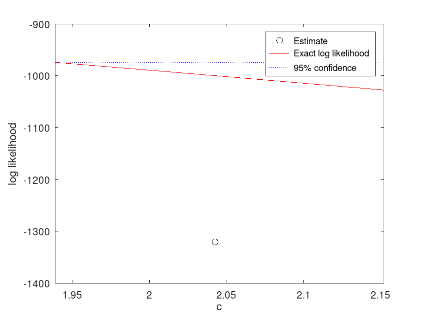
Use this to analyze the profile likelihood of the first shape parameter (c), helping to understand the uncertainty in parameter estimates for models like household income.
BurrDistribution: r = random (pd)
BurrDistribution: r = random (pd, rows)
BurrDistribution: r = random (pd, rows, cols, …)
BurrDistribution: r = random (pd, [sz])
r = random (pd) returns a random number from the
distribution object pd.
When called with a single size argument, burrrnd returns a square
matrix with the dimension specified. When called with more than one
scalar argument, the first two arguments are taken as the number of rows
and columns and any further arguments specify additional matrix
dimensions. The size may also be specified with a row vector of
dimensions, sz.
Example: 1
Generate random samples from a Burr distribution
pd = makedist ("Burr", "alpha", 1, "c", 2, "k", 3)
pd =
  BurrDistribution

  Burr distribution
    alpha = 1
        c = 2
        k = 3
 rand ("seed", 21);
 samples = random (pd, 50, 1);
 hist (samples, 90)
 title ("Histogram of 50 random samples from Burr(alpha=1, c=2, k=3)")
 xlabel ("values in x")
 ylabel ("Frequency")
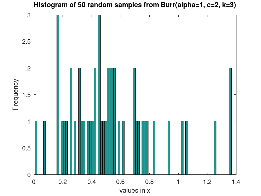
This generates random samples from a Burr distribution, useful for simulating non-negative data like household income under specific parameters.
BurrDistribution: s = std (pd)
s = std (pd) computes the standard deviation of the
probability distribution object, pd.
Example: 1
Compute the standard deviation for a Burr distribution
pd = makedist ("Burr", "alpha", 1, "c", 2, "k", 1)
pd =
  BurrDistribution

  Burr distribution
    alpha = 1
        c = 2
        k = 1
std_value = std (pd)
std_value = Inf
Use this to calculate the standard deviation, which measures the variability in the distribution, e.g., spread of household income.
BurrDistribution: t = truncate (pd, lower, upper)
t = truncate (pd, lower, upper) returns a
probability distribution t, which is the probability distribution
pd truncated to the specified interval with lower limit,
lower,
and upper limit, upper. If pd is fitted to data with
fitdist, the returned probability distribution t is not
fitted, does not contain any data or estimated values, and it is as it
has been created with the makedist function, but it includes the
truncation interval.
Example: 1
Plot the PDF of a Burr distribution, with parameters alpha = 1, c = 2, k = 1, truncated at [0.5, 2.5] intervals. Generate 10000 random samples from this truncated distribution and superimpose a histogram scaled accordingly
pd = makedist ("Burr", "alpha", 1, "c", 2, "k", 1)
pd =
  BurrDistribution

  Burr distribution
    alpha = 1
        c = 2
        k = 1
t = truncate (pd, 0.5, 2.5)
t =
  BurrDistribution

  Burr distribution
    alpha = 1
        c = 2
        k = 1
  Truncated to the interval [0.5, 2.5]
 rand ("seed", 21);
 data = random (t, 10000, 1);
Plot histogram and fitted PDF
 plot (t)
 hold on
 hist (data, 100, 50)
 hold off
 title ("Burr distribution (alpha = 1, c = 2, k = 1) truncated at [0.5, 2.5]")
 legend ("Truncated PDF", "Histogram")
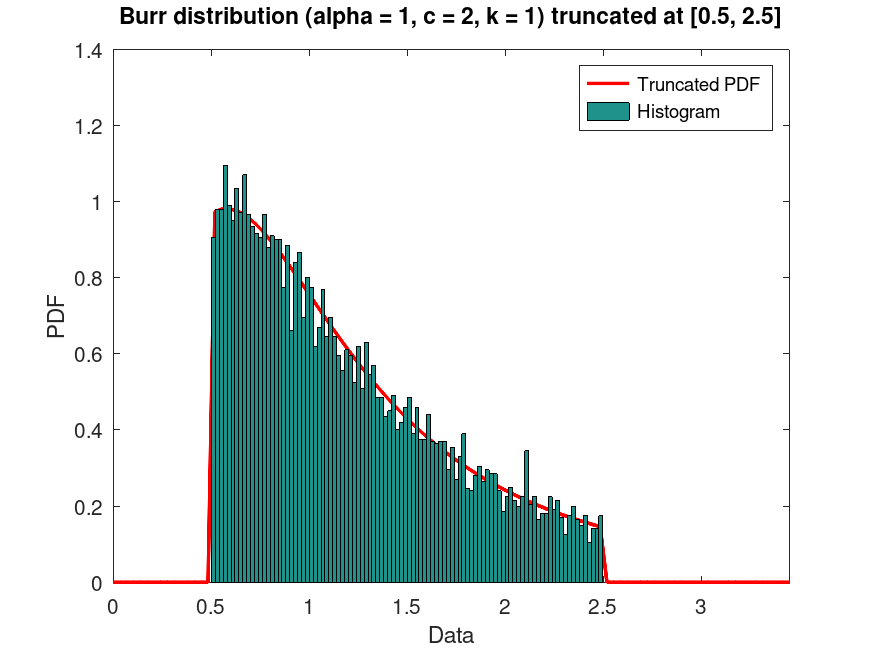
This demonstrates truncating a Burr distribution to a specific range and visualizing the resulting distribution with random samples, useful for bounded data scenarios.
BurrDistribution: v = var (pd)
v = var (pd) computes the variance of the
probability distribution object, pd.
Example: 1
Compute the variance for a Burr distribution
pd = makedist ("Burr", "alpha", 1, "c", 2, "k", 1)
pd =
  BurrDistribution

  Burr distribution
    alpha = 1
        c = 2
        k = 1
var_value = var (pd)
var_value = Inf
Use this to calculate the variance, which quantifies the spread of the distribution, e.g., variability in household income.
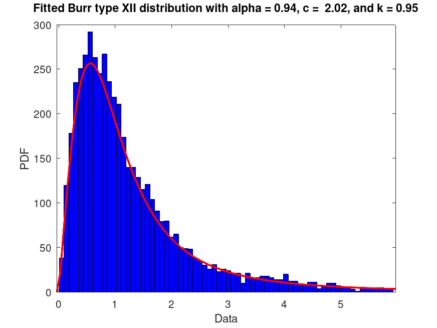
Examples
pd = makedist ('Burr', 'alpha', 1, 'c', 2, 'k', 1)
pd =
  BurrDistribution

  Burr distribution
    alpha = 1
        c = 2
        k = 1
 rand ('seed', 21);
 data = random (pd, 5000, 1);
 pd = fitdist (data, 'Burr')
pd =
  BurrDistribution

  Burr distribution
    alpha = 0.943213   [0.920634, 0.966345]
        c =  2.01899   [1.9726, 2.06648]
        k = 0.946371   [0.857098, 1.04494]
 plot (pd)
 msg = strcat ("Fitted Burr type XII distribution with", ...
               " alpha = %0.2f, c =  %0.2f, and k = %0.2f");
 title (sprintf (msg, pd.alpha, pd.c, pd.k))