Categories &
Functions List
- BetaDistribution
- BinomialDistribution
- BirnbaumSaundersDistribution
- BurrDistribution
- ExponentialDistribution
- ExtremeValueDistribution
- GammaDistribution
- GeneralizedExtremeValueDistribution
- GeneralizedParetoDistribution
- HalfNormalDistribution
- InverseGaussianDistribution
- LogisticDistribution
- LoglogisticDistribution
- LognormalDistribution
- LoguniformDistribution
- MultinomialDistribution
- NakagamiDistribution
- NegativeBinomialDistribution
- NormalDistribution
- PiecewiseLinearDistribution
- PoissonDistribution
- RayleighDistribution
- RicianDistribution
- tLocationScaleDistribution
- TriangularDistribution
- UniformDistribution
- WeibullDistribution
- betafit
- betalike
- binofit
- binolike
- bisafit
- bisalike
- burrfit
- burrlike
- evfit
- evlike
- expfit
- explike
- gamfit
- gamlike
- geofit
- gevfit_lmom
- gevfit
- gevlike
- gpfit
- gplike
- gumbelfit
- gumbellike
- hnfit
- hnlike
- invgfit
- invglike
- logifit
- logilike
- loglfit
- logllike
- lognfit
- lognlike
- nakafit
- nakalike
- nbinfit
- nbinlike
- normfit
- normlike
- poissfit
- poisslike
- raylfit
- rayllike
- ricefit
- ricelike
- tlsfit
- tlslike
- unidfit
- unifit
- wblfit
- wbllike
- betacdf
- betainv
- betapdf
- betarnd
- binocdf
- binoinv
- binopdf
- binornd
- bisacdf
- bisainv
- bisapdf
- bisarnd
- burrcdf
- burrinv
- burrpdf
- burrrnd
- bvncdf
- bvtcdf
- cauchycdf
- cauchyinv
- cauchypdf
- cauchyrnd
- chi2cdf
- chi2inv
- chi2pdf
- chi2rnd
- copulacdf
- copulapdf
- copularnd
- evcdf
- evinv
- evpdf
- evrnd
- expcdf
- expinv
- exppdf
- exprnd
- fcdf
- finv
- fpdf
- frnd
- gamcdf
- gaminv
- gampdf
- gamrnd
- geocdf
- geoinv
- geopdf
- geornd
- gevcdf
- gevinv
- gevpdf
- gevrnd
- gpcdf
- gpinv
- gppdf
- gprnd
- gumbelcdf
- gumbelinv
- gumbelpdf
- gumbelrnd
- hncdf
- hninv
- hnpdf
- hnrnd
- hygecdf
- hygeinv
- hygepdf
- hygernd
- invgcdf
- invginv
- invgpdf
- invgrnd
- iwishpdf
- iwishrnd
- jsucdf
- jsupdf
- laplacecdf
- laplaceinv
- laplacepdf
- laplacernd
- logicdf
- logiinv
- logipdf
- logirnd
- loglcdf
- loglinv
- loglpdf
- loglrnd
- logncdf
- logninv
- lognpdf
- lognrnd
- mnpdf
- mnrnd
- mvncdf
- mvnpdf
- mvnrnd
- mvtcdf
- mvtpdf
- mvtrnd
- mvtcdfqmc
- nakacdf
- nakainv
- nakapdf
- nakarnd
- nbincdf
- nbininv
- nbinpdf
- nbinrnd
- ncfcdf
- ncfinv
- ncfpdf
- ncfrnd
- nctcdf
- nctinv
- nctpdf
- nctrnd
- ncx2cdf
- ncx2inv
- ncx2pdf
- ncx2rnd
- normcdf
- norminv
- normpdf
- normrnd
- plcdf
- plinv
- plpdf
- plrnd
- poisscdf
- poissinv
- poisspdf
- poissrnd
- raylcdf
- raylinv
- raylpdf
- raylrnd
- ricecdf
- riceinv
- ricepdf
- ricernd
- tcdf
- tinv
- tpdf
- trnd
- tlscdf
- tlsinv
- tlspdf
- tlsrnd
- tricdf
- triinv
- tripdf
- trirnd
- unidcdf
- unidinv
- unidpdf
- unidrnd
- unifcdf
- unifinv
- unifpdf
- unifrnd
- vmcdf
- vminv
- vmpdf
- vmrnd
- wblcdf
- wblinv
- wblpdf
- wblrnd
- wienrnd
- wishpdf
- wishrnd
- adtest
- anova
- anova1
- anova2
- anovan
- bartlett_test
- barttest
- binotest
- chi2gof
- chi2test
- correlation_test
- fishertest
- friedman
- hotelling_t2test
- hotelling_t2test2
- kruskalwallis
- kstest
- kstest2
- levene_test
- manova1
- mcnemar_test
- multcompare
- ranksum
- regression_ftest
- regression_ttest
- runstest
- sampsizepwr
- signrank
- signtest
- tiedrank
- ttest
- ttest2
- vartest
- vartest2
- vartestn
- ztest
- ztest2
Function Reference: burrfit
statistics: paramhat = burrfit (x)
statistics: [paramhat, paramci] = burrfit (x)
statistics: [paramhat, paramci] = burrfit (x, alpha)
statistics: […] = burrfit (x, alpha, censor)
statistics: […] = burrfit (x, alpha, censor, freq)
statistics: […] = burrfit (x, alpha, censor, freq, options)
Estimate mean and confidence intervals for the Burr type XII distribution.
muhat = burrfit (x) returns the maximum likelihood
estimates of the parameters of the Burr type XII distribution given the data
in x. paramhat(1) is the scale parameter, lambda,
paramhat(2) is the first shape parameter, c, and
paramhat(3) is the second shape parameter, k
[paramhat, paramci] = burrfit (x) returns the 95%
confidence intervals for the parameter estimates.
[…] = burrfit (x, alpha) also returns the
100 * (1 - alpha) percent confidence intervals for the
parameter estimates. By default, the optional argument alpha is
0.05 corresponding to 95% confidence intervals. Pass in [] for
alpha to use the default values.
[…] = burrfit (x, alpha, censor) accepts a
boolean vector, censor, of the same size as x with 1s for
observations that are right-censored and 0s for observations that are
observed exactly. By default, or if left empty,
censor = zeros (size (x)).
[…] = burrfit (x, alpha, censor, freq)
accepts a frequency vector, freq, of the same size as x.
freq typically contains integer frequencies for the corresponding
elements in x, but it can contain any non-integer non-negative values.
By default, or if left empty, freq = ones (size (x)).
[…] = burrfit (…, options) specifies control
parameters for the iterative algorithm used to compute the maximum likelihood
estimates. options is a structure with the following field and its
default value:
-
options.Display = "off" -
options.MaxFunEvals = 400 -
options.MaxIter = 200 -
options.TolX = 1e-6
Further information about the Burr type XII distribution can be found at https://en.wikipedia.org/wiki/Burr_distribution
See also: burrcdf, burrinv, burrpdf, burrrnd, burrlike, burrstat
Source Code: burrfit
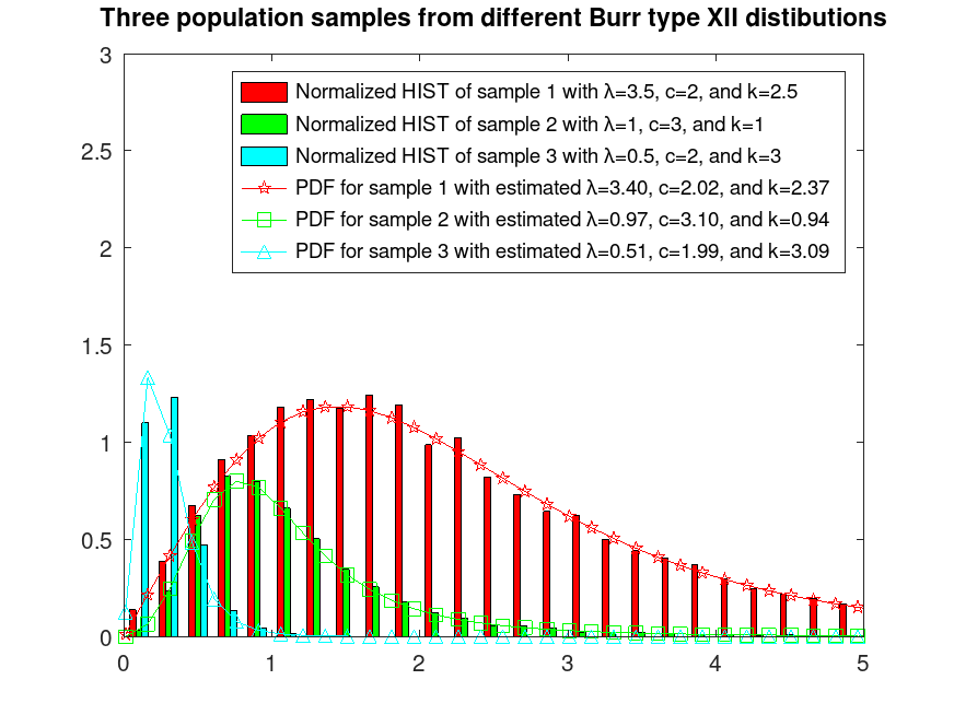
Example: 1
Sample 3 populations from different Burr type XII distributions
 rand ('seed', 4);    # for reproducibility
 r1 = burrrnd (3.5, 2, 2.5, 10000, 1);
 rand ('seed', 2);    # for reproducibility
 r2 = burrrnd (1, 3, 1, 10000, 1);
 rand ('seed', 9);    # for reproducibility
 r3 = burrrnd (0.5, 2, 3, 10000, 1);
 r = [r1, r2, r3];
Plot them normalized and fix their colors
 hist (r, [0.1:0.2:20], [18, 5, 3]);
 h = findobj (gca, 'Type', 'patch');
 set (h(1), 'facecolor', 'c');
 set (h(2), 'facecolor', 'g');
 set (h(3), 'facecolor', 'r');
 ylim ([0, 3]);
 xlim ([0, 5]);
 hold on
Estimate their α and β parameters
 lambda_c_kA = burrfit (r(:,1));
 lambda_c_kB = burrfit (r(:,2));
 lambda_c_kC = burrfit (r(:,3));
Plot their estimated PDFs
 x = [0.01:0.15:15];
 y = burrpdf (x, lambda_c_kA(1), lambda_c_kA(2), lambda_c_kA(3));
 plot (x, y, '-pr');
 y = burrpdf (x, lambda_c_kB(1), lambda_c_kB(2), lambda_c_kB(3));
 plot (x, y, '-sg');
 y = burrpdf (x, lambda_c_kC(1), lambda_c_kC(2), lambda_c_kC(3));
 plot (x, y, '-^c');
 hold off
 legend ({'Normalized HIST of sample 1 with λ=3.5, c=2, and k=2.5', ...
          'Normalized HIST of sample 2 with λ=1, c=3, and k=1', ...
          'Normalized HIST of sample 3 with λ=0.5, c=2, and k=3', ...
  sprintf("PDF for sample 1 with estimated λ=%0.2f, c=%0.2f, and k=%0.2f", ...
          lambda_c_kA(1), lambda_c_kA(2), lambda_c_kA(3)), ...
  sprintf("PDF for sample 2 with estimated λ=%0.2f, c=%0.2f, and k=%0.2f", ...
          lambda_c_kB(1), lambda_c_kB(2), lambda_c_kB(3)), ...
  sprintf("PDF for sample 3 with estimated λ=%0.2f, c=%0.2f, and k=%0.2f", ...
          lambda_c_kC(1), lambda_c_kC(2), lambda_c_kC(3))})
 title ('Three population samples from different Burr type XII distributions')
 hold off