Categories &
Functions List
- BetaDistribution
- BinomialDistribution
- BirnbaumSaundersDistribution
- BurrDistribution
- ExponentialDistribution
- ExtremeValueDistribution
- GammaDistribution
- GeneralizedExtremeValueDistribution
- GeneralizedParetoDistribution
- HalfNormalDistribution
- InverseGaussianDistribution
- LogisticDistribution
- LoglogisticDistribution
- LognormalDistribution
- LoguniformDistribution
- MultinomialDistribution
- NakagamiDistribution
- NegativeBinomialDistribution
- NormalDistribution
- PiecewiseLinearDistribution
- PoissonDistribution
- RayleighDistribution
- RicianDistribution
- tLocationScaleDistribution
- TriangularDistribution
- UniformDistribution
- WeibullDistribution
- betafit
- betalike
- binofit
- binolike
- bisafit
- bisalike
- burrfit
- burrlike
- evfit
- evlike
- expfit
- explike
- gamfit
- gamlike
- geofit
- gevfit_lmom
- gevfit
- gevlike
- gpfit
- gplike
- gumbelfit
- gumbellike
- hnfit
- hnlike
- invgfit
- invglike
- logifit
- logilike
- loglfit
- logllike
- lognfit
- lognlike
- nakafit
- nakalike
- nbinfit
- nbinlike
- normfit
- normlike
- poissfit
- poisslike
- raylfit
- rayllike
- ricefit
- ricelike
- tlsfit
- tlslike
- unidfit
- unifit
- wblfit
- wbllike
- betacdf
- betainv
- betapdf
- betarnd
- binocdf
- binoinv
- binopdf
- binornd
- bisacdf
- bisainv
- bisapdf
- bisarnd
- burrcdf
- burrinv
- burrpdf
- burrrnd
- bvncdf
- bvtcdf
- cauchycdf
- cauchyinv
- cauchypdf
- cauchyrnd
- chi2cdf
- chi2inv
- chi2pdf
- chi2rnd
- copulacdf
- copulapdf
- copularnd
- evcdf
- evinv
- evpdf
- evrnd
- expcdf
- expinv
- exppdf
- exprnd
- fcdf
- finv
- fpdf
- frnd
- gamcdf
- gaminv
- gampdf
- gamrnd
- geocdf
- geoinv
- geopdf
- geornd
- gevcdf
- gevinv
- gevpdf
- gevrnd
- gpcdf
- gpinv
- gppdf
- gprnd
- gumbelcdf
- gumbelinv
- gumbelpdf
- gumbelrnd
- hncdf
- hninv
- hnpdf
- hnrnd
- hygecdf
- hygeinv
- hygepdf
- hygernd
- invgcdf
- invginv
- invgpdf
- invgrnd
- iwishpdf
- iwishrnd
- jsucdf
- jsupdf
- laplacecdf
- laplaceinv
- laplacepdf
- laplacernd
- logicdf
- logiinv
- logipdf
- logirnd
- loglcdf
- loglinv
- loglpdf
- loglrnd
- logncdf
- logninv
- lognpdf
- lognrnd
- mnpdf
- mnrnd
- mvncdf
- mvnpdf
- mvnrnd
- mvtcdf
- mvtpdf
- mvtrnd
- mvtcdfqmc
- nakacdf
- nakainv
- nakapdf
- nakarnd
- nbincdf
- nbininv
- nbinpdf
- nbinrnd
- ncfcdf
- ncfinv
- ncfpdf
- ncfrnd
- nctcdf
- nctinv
- nctpdf
- nctrnd
- ncx2cdf
- ncx2inv
- ncx2pdf
- ncx2rnd
- normcdf
- norminv
- normpdf
- normrnd
- plcdf
- plinv
- plpdf
- plrnd
- poisscdf
- poissinv
- poisspdf
- poissrnd
- raylcdf
- raylinv
- raylpdf
- raylrnd
- ricecdf
- riceinv
- ricepdf
- ricernd
- tcdf
- tinv
- tpdf
- trnd
- tlscdf
- tlsinv
- tlspdf
- tlsrnd
- tricdf
- triinv
- tripdf
- trirnd
- unidcdf
- unidinv
- unidpdf
- unidrnd
- unifcdf
- unifinv
- unifpdf
- unifrnd
- vmcdf
- vminv
- vmpdf
- vmrnd
- wblcdf
- wblinv
- wblpdf
- wblrnd
- wienrnd
- wishpdf
- wishrnd
- adtest
- anova
- anova1
- anova2
- anovan
- bartlett_test
- barttest
- binotest
- chi2gof
- chi2test
- correlation_test
- fishertest
- friedman
- hotelling_t2test
- hotelling_t2test2
- kruskalwallis
- kstest
- kstest2
- levene_test
- manova1
- mcnemar_test
- multcompare
- ranksum
- regression_ftest
- regression_ttest
- runstest
- sampsizepwr
- signrank
- signtest
- tiedrank
- ttest
- ttest2
- vartest
- vartest2
- vartestn
- ztest
- ztest2
Function Reference: loglfit
statistics: paramhat = loglfit (x)
statistics: [paramhat, paramci] = loglfit (x)
statistics: [paramhat, paramci] = loglfit (x, alpha)
statistics: […] = loglfit (x, alpha, censor)
statistics: […] = loglfit (x, alpha, censor, freq)
statistics: […] = loglfit (x, alpha, censor, freq, options)
Estimate mean and confidence intervals for the log-logistic distribution.
mu0 = loglfit (x) returns the maximum likelihood
estimates of the parameters of the log-logistic distribution given the data
in x. paramhat(1) is the mean parameter, mu, and
paramhat(2) is the scale parameter, sigma.
[paramhat, paramci] = loglfit (x) returns the 95%
confidence intervals for the parameter estimates.
[…] = loglfit (x, alpha) also returns the
100 * (1 - alpha) percent confidence intervals for the
parameter estimates. By default, the optional argument alpha is
0.05 corresponding to 95% confidence intervals. Pass in [] for
alpha to use the default values.
[…] = loglfit (x, alpha, censor) accepts a
boolean vector, censor, of the same size as x with 1s for
observations that are right-censored and 0s for observations that are
observed exactly. By default, or if left empty,
censor = zeros (size (x)).
[…] = loglfit (x, alpha, censor, freq)
accepts a frequency vector, freq, of the same size as x.
freq typically contains integer frequencies for the corresponding
elements in x, but it can contain any non-integer non-negative values.
By default, or if left empty, freq = ones (size (x)).
[…] = loglfit (…, options) specifies control
parameters for the iterative algorithm used to compute ML estimates with the
fminsearch function. options is a structure with the following
fields and their default values:
-
options.Display = "off" -
options.MaxFunEvals = 400 -
options.MaxIter = 200 -
options.TolX = 1e-6
Further information about the loglogistic distribution can be found at https://en.wikipedia.org/wiki/Log-logistic_distribution
OCTAVE/MATLAB use an alternative parameterization given by the pair , i.e. mu and sigma, in analogy with the logistic distribution. Their relation to the and parameters used in Wikipedia are given below:
-
mu = log (a) -
sigma = 1 / a
See also: loglcdf, loglinv, loglpdf, loglrnd, logllike, loglstat
Source Code: loglfit
Example: 1
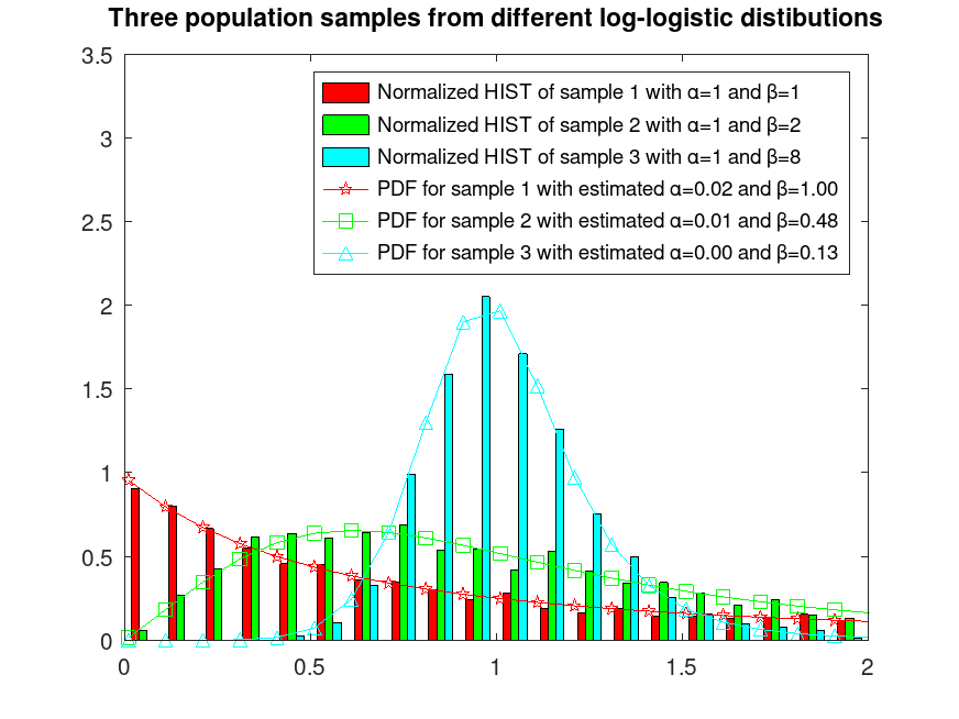
Sample 3 populations from different log-logistic distributions
 rand ('seed', 5)  # for reproducibility
 r1 = loglrnd (0, 1, 2000, 1);
 rand ('seed', 2)   # for reproducibility
 r2 = loglrnd (0, 0.5, 2000, 1);
 rand ('seed', 7)   # for reproducibility
 r3 = loglrnd (0, 0.125, 2000, 1);
 r = [r1, r2, r3];
Plot them normalized and fix their colors
 hist (r, [0.05:0.1:2.5], 10);
 h = findobj (gca, 'Type', 'patch');
 set (h(1), 'facecolor', 'c');
 set (h(2), 'facecolor', 'g');
 set (h(3), 'facecolor', 'r');
 ylim ([0, 3.5]);
 xlim ([0, 2.0]);
 hold on
Estimate their MU and LAMBDA parameters
 a_bA = loglfit (r(:,1));
 a_bB = loglfit (r(:,2));
 a_bC = loglfit (r(:,3));
Plot their estimated PDFs
 x = [0.01:0.1:2.01];
 y = loglpdf (x, a_bA(1), a_bA(2));
 plot (x, y, '-pr');
 y = loglpdf (x, a_bB(1), a_bB(2));
 plot (x, y, '-sg');
 y = loglpdf (x, a_bC(1), a_bC(2));
 plot (x, y, '-^c');
 legend ({'Normalized HIST of sample 1 with α=1 and β=1', ...
          'Normalized HIST of sample 2 with α=1 and β=2', ...
          'Normalized HIST of sample 3 with α=1 and β=8', ...
          sprintf("PDF for sample 1 with estimated α=%0.2f and β=%0.2f", ...
                  a_bA(1), a_bA(2)), ...
          sprintf("PDF for sample 2 with estimated α=%0.2f and β=%0.2f", ...
                  a_bB(1), a_bB(2)), ...
          sprintf("PDF for sample 3 with estimated α=%0.2f and β=%0.2f", ...
                  a_bC(1), a_bC(2))})
 title ('Three population samples from different log-logistic distributions')
 hold off