Categories &
Functions List
- BetaDistribution
- BinomialDistribution
- BirnbaumSaundersDistribution
- BurrDistribution
- ExponentialDistribution
- ExtremeValueDistribution
- GammaDistribution
- GeneralizedExtremeValueDistribution
- GeneralizedParetoDistribution
- HalfNormalDistribution
- InverseGaussianDistribution
- LogisticDistribution
- LoglogisticDistribution
- LognormalDistribution
- LoguniformDistribution
- MultinomialDistribution
- NakagamiDistribution
- NegativeBinomialDistribution
- NormalDistribution
- PiecewiseLinearDistribution
- PoissonDistribution
- RayleighDistribution
- RicianDistribution
- tLocationScaleDistribution
- TriangularDistribution
- UniformDistribution
- WeibullDistribution
- betafit
- betalike
- binofit
- binolike
- bisafit
- bisalike
- burrfit
- burrlike
- evfit
- evlike
- expfit
- explike
- gamfit
- gamlike
- geofit
- gevfit_lmom
- gevfit
- gevlike
- gpfit
- gplike
- gumbelfit
- gumbellike
- hnfit
- hnlike
- invgfit
- invglike
- logifit
- logilike
- loglfit
- logllike
- lognfit
- lognlike
- nakafit
- nakalike
- nbinfit
- nbinlike
- normfit
- normlike
- poissfit
- poisslike
- raylfit
- rayllike
- ricefit
- ricelike
- tlsfit
- tlslike
- unidfit
- unifit
- wblfit
- wbllike
- betacdf
- betainv
- betapdf
- betarnd
- binocdf
- binoinv
- binopdf
- binornd
- bisacdf
- bisainv
- bisapdf
- bisarnd
- burrcdf
- burrinv
- burrpdf
- burrrnd
- bvncdf
- bvtcdf
- cauchycdf
- cauchyinv
- cauchypdf
- cauchyrnd
- chi2cdf
- chi2inv
- chi2pdf
- chi2rnd
- copulacdf
- copulapdf
- copularnd
- evcdf
- evinv
- evpdf
- evrnd
- expcdf
- expinv
- exppdf
- exprnd
- fcdf
- finv
- fpdf
- frnd
- gamcdf
- gaminv
- gampdf
- gamrnd
- geocdf
- geoinv
- geopdf
- geornd
- gevcdf
- gevinv
- gevpdf
- gevrnd
- gpcdf
- gpinv
- gppdf
- gprnd
- gumbelcdf
- gumbelinv
- gumbelpdf
- gumbelrnd
- hncdf
- hninv
- hnpdf
- hnrnd
- hygecdf
- hygeinv
- hygepdf
- hygernd
- invgcdf
- invginv
- invgpdf
- invgrnd
- iwishpdf
- iwishrnd
- jsucdf
- jsupdf
- laplacecdf
- laplaceinv
- laplacepdf
- laplacernd
- logicdf
- logiinv
- logipdf
- logirnd
- loglcdf
- loglinv
- loglpdf
- loglrnd
- logncdf
- logninv
- lognpdf
- lognrnd
- mnpdf
- mnrnd
- mvncdf
- mvnpdf
- mvnrnd
- mvtcdf
- mvtpdf
- mvtrnd
- mvtcdfqmc
- nakacdf
- nakainv
- nakapdf
- nakarnd
- nbincdf
- nbininv
- nbinpdf
- nbinrnd
- ncfcdf
- ncfinv
- ncfpdf
- ncfrnd
- nctcdf
- nctinv
- nctpdf
- nctrnd
- ncx2cdf
- ncx2inv
- ncx2pdf
- ncx2rnd
- normcdf
- norminv
- normpdf
- normrnd
- plcdf
- plinv
- plpdf
- plrnd
- poisscdf
- poissinv
- poisspdf
- poissrnd
- raylcdf
- raylinv
- raylpdf
- raylrnd
- ricecdf
- riceinv
- ricepdf
- ricernd
- tcdf
- tinv
- tpdf
- trnd
- tlscdf
- tlsinv
- tlspdf
- tlsrnd
- tricdf
- triinv
- tripdf
- trirnd
- unidcdf
- unidinv
- unidpdf
- unidrnd
- unifcdf
- unifinv
- unifpdf
- unifrnd
- vmcdf
- vminv
- vmpdf
- vmrnd
- wblcdf
- wblinv
- wblpdf
- wblrnd
- wienrnd
- wishpdf
- wishrnd
- adtest
- anova
- anova1
- anova2
- anovan
- bartlett_test
- barttest
- binotest
- chi2gof
- chi2test
- correlation_test
- fishertest
- friedman
- hotelling_t2test
- hotelling_t2test2
- kruskalwallis
- kstest
- kstest2
- levene_test
- manova1
- mcnemar_test
- multcompare
- ranksum
- regression_ftest
- regression_ttest
- runstest
- sampsizepwr
- signrank
- signtest
- tiedrank
- ttest
- ttest2
- vartest
- vartest2
- vartestn
- ztest
- ztest2
Function Reference: slicesample
statistics: [smpl, neval] = slicesample (start, nsamples, property, value, …)
Draws nsamples samples from a target stationary distribution pdf using slice sampling of Radford M. Neal.
Input:
- start is a 1 by dim vector of the starting point of the Markov chain. Each column corresponds to a different dimension.
- nsamples is the number of samples, the length of the Markov chain.
Next, several property-value pairs can or must be specified, they are:
(Required properties) One of:
-
"pdf": the value is a function handle of the target stationary
distribution to be sampled. The function should accept different locations
in each row and each column corresponds to a different dimension.
or
- logpdf: the value is a function handle of the log of the target stationary distribution to be sampled. The function should accept different locations in each row and each column corresponds to a different dimension.
The following input property/pair values may be needed depending on the desired output:
- "burnin" burnin the number of points to discard at the beginning, the default is 0.
- "thin" thin omits m-1 of every m points in the generated Markov chain. The default is 1.
- "width" width the maximum Manhattan distance between two samples. The default is 10.
Outputs:
- smpl is a nsamples by dim matrix of random values drawn from pdf where the rows are different random values, the columns correspond to the dimensions of pdf.
- neval is the number of function evaluations per sample.
Example : Sampling from a normal distribution
start = 1; nsamples = 1e3; pdf = @(x) exp (-.5 * x .^ 2) / (pi ^ .5 * 2 ^ .5); [smpl, accept] = slicesample (start, nsamples, "pdf", pdf, "thin", 4); histfit (smpl); |
See also: rand, mhsample, randsample
Source Code: slicesample
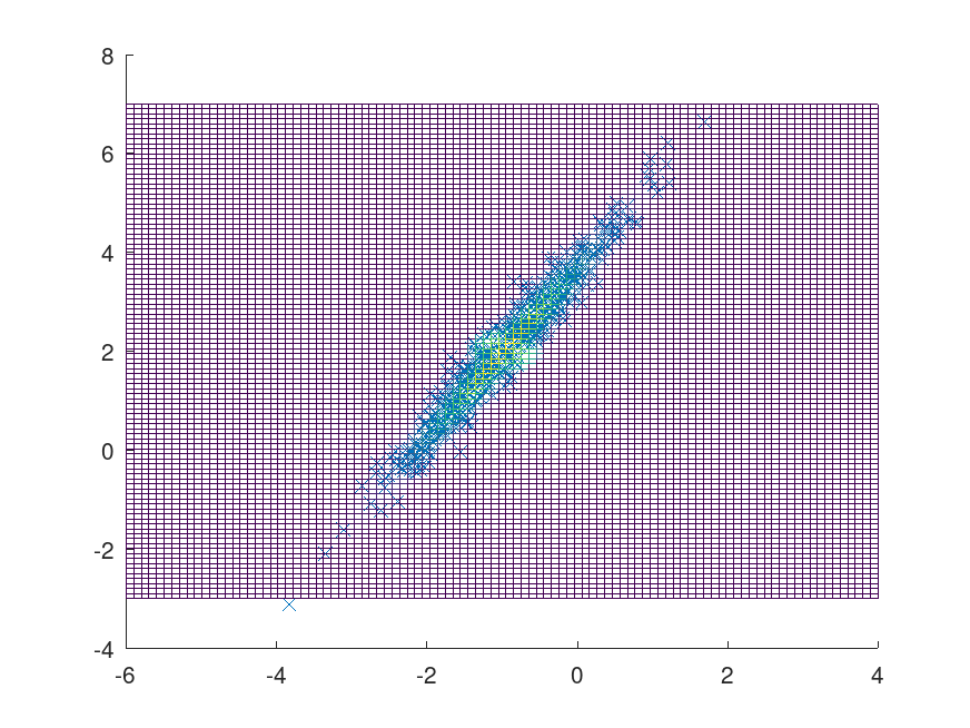
Example: 1
Define function to sample
 d = 2;
 mu = [-1; 2];
 rand ('seed', 5)  # for reproducibility
 Sigma = rand (d);
 Sigma = (Sigma + Sigma');
 Sigma += eye (d)*abs (eigs (Sigma, 1, 'sa')) * 1.1;
 pdf = @(x)(2*pi)^(-d/2)*det (Sigma)^-.5*exp (-.5*sum ((x.'-mu).*(Sigma\(x.'-mu)),1));
Inputs
 start = ones (1,2);
 nsamples = 500;
 K = 500;
 m = 10;
 rande ('seed', 4);  rand ('seed', 5)  # for reproducibility
 [smpl, accept] = slicesample (start, nsamples, 'pdf', pdf, 'burnin', K, 'thin', m, 'width', [20, 30]);
 figure;
 hold on;
 plot (smpl(:,1), smpl(:,2), 'x');
 [x, y] = meshgrid (linspace (-6,4), linspace (-3,7));
 z = reshape (pdf ([x(:), y(:)]), size (x));
 mesh (x, y, z, 'facecolor', 'None');
Using sample points to find the volume of half a sphere with radius of .5
 f = @(x) ((.25-(x(:,1)+1).^2-(x(:,2)-2).^2).^.5.*(((x(:,1)+1).^2+(x(:,2)-2).^2)<.25)).';
 int = mean (f(smpl) ./ pdf (smpl));
 errest = std (f(smpl) ./ pdf (smpl)) / nsamples^.5;
 trueerr = abs (2/3*pi*.25^(3/2)-int);
 fprintf ("Monte Carlo integral estimate int f(x) dx = %f\n", int);
Monte Carlo integral estimate int f(x) dx = 0.228408
fprintf ("Monte Carlo integral error estimate %f\n", errest);
Monte Carlo integral error estimate 0.029831
fprintf ("The actual error %f\n", trueerr);
The actual error 0.033392
mesh (x,y,reshape (f([x(:), y(:)]), size (x)), 'facecolor', 'None');
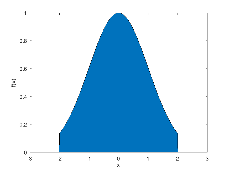
Example: 2
Integrate truncated normal distribution to find normalization constant
 pdf = @(x) exp (-.5*x.^2)/(pi^.5*2^.5);
 nsamples = 1e3;
 rande ('seed', 4);  rand ('seed', 5)  # for reproducibility
 [smpl, accept] = slicesample (1, nsamples, 'pdf', pdf, 'thin', 4);
 f = @(x) exp (-.5 * x .^ 2) .* (x >= -2 & x <= 2);
 x = linspace (-3, 3, 1000);
 area (x, f(x));
 xlabel ('x');
 ylabel ('f(x)');
 int = mean (f(smpl) ./ pdf (smpl));
 errest = std (f(smpl) ./ pdf (smpl)) / nsamples ^ 0.5;
 trueerr = abs (erf (2 ^ 0.5) * 2 ^ 0.5 * pi ^ 0.5 - int);
 fprintf ("Monte Carlo integral estimate int f(x) dx = %f\n", int);
Monte Carlo integral estimate int f(x) dx = 2.376284
fprintf ("Monte Carlo integral error estimate %f\n", errest);
Monte Carlo integral error estimate 0.017608
fprintf ("The actual error %f\n", trueerr);
The actual error 0.016292