Categories &
Functions List
- BetaDistribution
- BinomialDistribution
- BirnbaumSaundersDistribution
- BurrDistribution
- ExponentialDistribution
- ExtremeValueDistribution
- GammaDistribution
- GeneralizedExtremeValueDistribution
- GeneralizedParetoDistribution
- HalfNormalDistribution
- InverseGaussianDistribution
- LogisticDistribution
- LoglogisticDistribution
- LognormalDistribution
- LoguniformDistribution
- MultinomialDistribution
- NakagamiDistribution
- NegativeBinomialDistribution
- NormalDistribution
- PiecewiseLinearDistribution
- PoissonDistribution
- RayleighDistribution
- RicianDistribution
- tLocationScaleDistribution
- TriangularDistribution
- UniformDistribution
- WeibullDistribution
- betafit
- betalike
- binofit
- binolike
- bisafit
- bisalike
- burrfit
- burrlike
- evfit
- evlike
- expfit
- explike
- gamfit
- gamlike
- geofit
- gevfit_lmom
- gevfit
- gevlike
- gpfit
- gplike
- gumbelfit
- gumbellike
- hnfit
- hnlike
- invgfit
- invglike
- logifit
- logilike
- loglfit
- logllike
- lognfit
- lognlike
- nakafit
- nakalike
- nbinfit
- nbinlike
- normfit
- normlike
- poissfit
- poisslike
- raylfit
- rayllike
- ricefit
- ricelike
- tlsfit
- tlslike
- unidfit
- unifit
- wblfit
- wbllike
- betacdf
- betainv
- betapdf
- betarnd
- binocdf
- binoinv
- binopdf
- binornd
- bisacdf
- bisainv
- bisapdf
- bisarnd
- burrcdf
- burrinv
- burrpdf
- burrrnd
- bvncdf
- bvtcdf
- cauchycdf
- cauchyinv
- cauchypdf
- cauchyrnd
- chi2cdf
- chi2inv
- chi2pdf
- chi2rnd
- copulacdf
- copulapdf
- copularnd
- evcdf
- evinv
- evpdf
- evrnd
- expcdf
- expinv
- exppdf
- exprnd
- fcdf
- finv
- fpdf
- frnd
- gamcdf
- gaminv
- gampdf
- gamrnd
- geocdf
- geoinv
- geopdf
- geornd
- gevcdf
- gevinv
- gevpdf
- gevrnd
- gpcdf
- gpinv
- gppdf
- gprnd
- gumbelcdf
- gumbelinv
- gumbelpdf
- gumbelrnd
- hncdf
- hninv
- hnpdf
- hnrnd
- hygecdf
- hygeinv
- hygepdf
- hygernd
- invgcdf
- invginv
- invgpdf
- invgrnd
- iwishpdf
- iwishrnd
- jsucdf
- jsupdf
- laplacecdf
- laplaceinv
- laplacepdf
- laplacernd
- logicdf
- logiinv
- logipdf
- logirnd
- loglcdf
- loglinv
- loglpdf
- loglrnd
- logncdf
- logninv
- lognpdf
- lognrnd
- mnpdf
- mnrnd
- mvncdf
- mvnpdf
- mvnrnd
- mvtcdf
- mvtpdf
- mvtrnd
- mvtcdfqmc
- nakacdf
- nakainv
- nakapdf
- nakarnd
- nbincdf
- nbininv
- nbinpdf
- nbinrnd
- ncfcdf
- ncfinv
- ncfpdf
- ncfrnd
- nctcdf
- nctinv
- nctpdf
- nctrnd
- ncx2cdf
- ncx2inv
- ncx2pdf
- ncx2rnd
- normcdf
- norminv
- normpdf
- normrnd
- plcdf
- plinv
- plpdf
- plrnd
- poisscdf
- poissinv
- poisspdf
- poissrnd
- raylcdf
- raylinv
- raylpdf
- raylrnd
- ricecdf
- riceinv
- ricepdf
- ricernd
- tcdf
- tinv
- tpdf
- trnd
- tlscdf
- tlsinv
- tlspdf
- tlsrnd
- tricdf
- triinv
- tripdf
- trirnd
- unidcdf
- unidinv
- unidpdf
- unidrnd
- unifcdf
- unifinv
- unifpdf
- unifrnd
- vmcdf
- vminv
- vmpdf
- vmrnd
- wblcdf
- wblinv
- wblpdf
- wblrnd
- wienrnd
- wishpdf
- wishrnd
- adtest
- anova
- anova1
- anova2
- anovan
- bartlett_test
- barttest
- binotest
- chi2gof
- chi2test
- correlation_test
- fishertest
- friedman
- hotelling_t2test
- hotelling_t2test2
- kruskalwallis
- kstest
- kstest2
- levene_test
- manova1
- mcnemar_test
- multcompare
- ranksum
- regression_ftest
- regression_ttest
- runstest
- sampsizepwr
- signrank
- signtest
- tiedrank
- ttest
- ttest2
- vartest
- vartest2
- vartestn
- ztest
- ztest2
Function Reference: regress_gp
statistics: [Yfit, Yint, m, K] = regress_gp (X, Y, Xfit)
statistics: [Yfit, Yint, m, K] = regress_gp (X, Y, Xfit,
'linear')statistics: [Yfit, Yint, Ysd] = regress_gp (X, Y, Xfit,
'rbf')statistics: […] = regress_gp (X, Y, Xfit,
'linear', Sp)statistics: […] = regress_gp (X, Y, Xfit, Sp)
statistics: […] = regress_gp (X, Y, Xfit,
'rbf', theta)statistics: […] = regress_gp (X, Y, Xfit,
'rbf', theta, g)statistics: […] = regress_gp (X, Y, Xfit,
'rbf', theta, g, alpha)statistics: […] = regress_gp (X, Y, Xfit, theta)
statistics: […] = regress_gp (X, Y, Xfit, theta, g)
statistics: […] = regress_gp (X, Y, Xfit, theta, g, alpha)
Regression using Gaussian Processes.
[Yfit, Yint, m, K] = regress_gp (X,
 Y, Xfit)
will estimate a linear Gaussian Process model m
in the form Y = X' * m, where X is an
matrix with observations in dimensional space
and Y is an column vector as the dependent variable. The
information about errors of the predictions (interpolation/extrapolation) is
given by the covariance matrix K.
By default, the linear model defines the prior covariance of m as
Sp = 100 * eye (size (X, 2) + 1). A custom prior
covariance matrix can be passed as Sp, which must be a
positive definite matrix. The model is evaluated for input Xfit, which
must have the same columns as X, and the estimates are returned in
Yfit along with the estimated variation in Yint.
Yint(:,1) contains the upper boundary estimate and
Yint(:,1) contains the upper boundary estimate with respect to
Yfit.
[Yfit, Yint, Ysd, K] = regress_gp (X,
Y, Xfit, will estimate a Gaussian Process model
with a Radial Basis Function (RBF) kernel with default parameters
'rbf')theta = 5, which corresponds to the characteristic lengthscale,
and g = 0.01, which corresponds to the nugget effect, and
alpha = 0.05 which defines the confidence level for the
estimated intervals returned in Yint. The function also returns the
predictive covariance matrix in Ysd. For multidimensional predictors
X the function will automatically normalize each column to a zero mean
and a standard deviation to one.
Run demo regress_gp to see examples.
See also: regress, regression_ftest, regression_ttest
Source Code: regress_gp
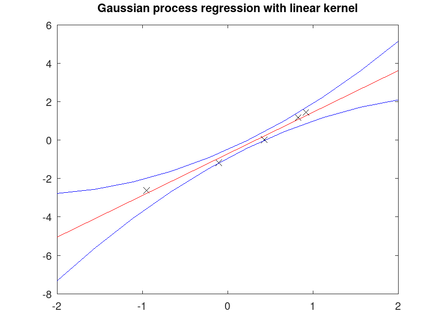
Example: 1
Linear fitting of 1D Data
 rand ('seed', 125);
 X = 2 * rand (5, 1) - 1;
 randn ('seed', 25);
 Y = 2 * X - 1 + 0.3 * randn (5, 1);
Points for interpolation/extrapolation
Xfit = linspace (-2, 2, 10)';
Fit regression model
[Yfit, Yint, m] = regress_gp (X, Y, Xfit);
Plot fitted data
 plot (X, Y, 'xk', Xfit, Yfit, 'r-', Xfit, Yint, 'b-');
 title ('Gaussian process regression with linear kernel');
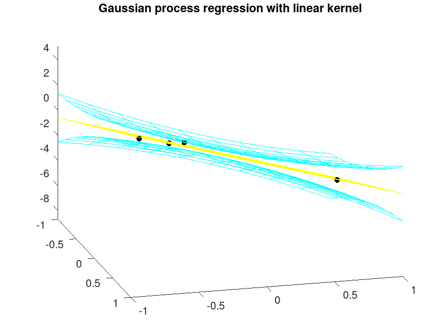
Example: 2
Linear fitting of 2D Data
 rand ('seed', 135);
 X = 2 * rand (4, 2) - 1;
 randn ('seed', 35);
 Y = 2 * X(:,1) - 3 * X(:,2) - 1 + 1 * randn (4, 1);
Mesh for interpolation/extrapolation
 [x1, x2] = meshgrid (linspace (-1, 1, 10));
 Xfit = [x1(:), x2(:)];
Fit regression model
 [Ypred, Yint, Ysd] = regress_gp (X, Y, Xfit);
 Ypred = reshape (Ypred, 10, 10);
 YintU = reshape (Yint(:,1), 10, 10);
 YintL = reshape (Yint(:,2), 10, 10);
Plot fitted data
 plot3 (X(:,1), X(:,2), Y, '.k', 'markersize', 16);
 hold on;
 h = mesh (x1, x2, Ypred, zeros (10, 10));
 set (h, 'facecolor', 'none', 'edgecolor', 'yellow');
 h = mesh (x1, x2, YintU, ones (10, 10));
 set (h, 'facecolor', 'none', 'edgecolor', 'cyan');
 h = mesh (x1, x2, YintL, ones (10, 10));
 set (h, 'facecolor', 'none', 'edgecolor', 'cyan');
 hold off
 axis tight
 view (75, 25)
 title ('Gaussian process regression with linear kernel');
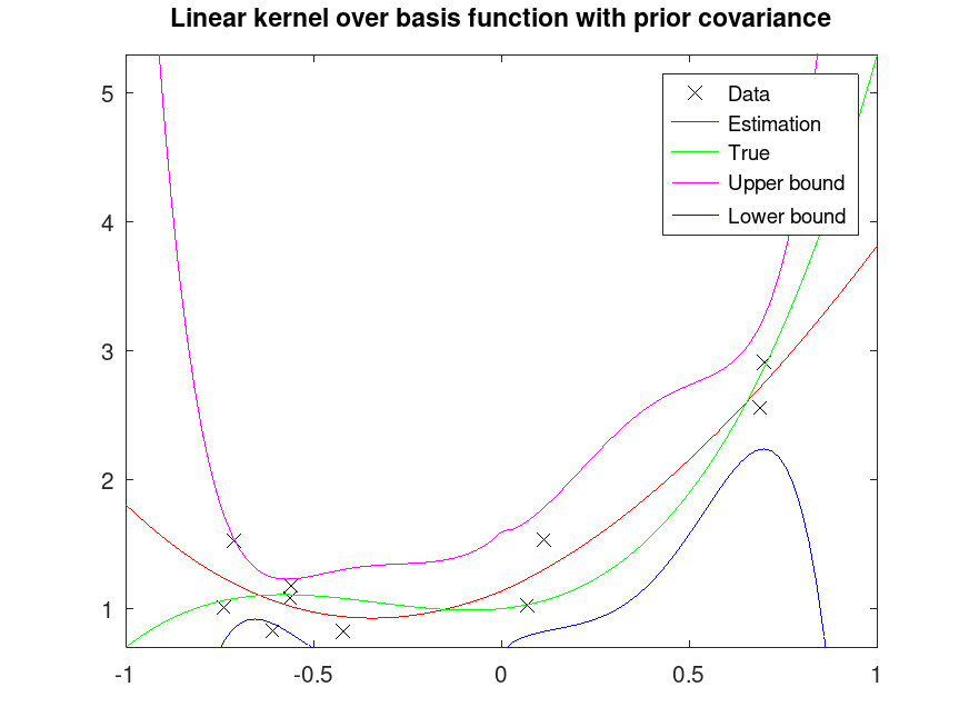
Example: 3
Projection over basis function with linear kernel
 pp = [2, 2, 0.3, 1];
 n = 10;
 rand ('seed', 145);
 X = 2 * rand (n, 1) - 1;
 randn ('seed', 45);
 Y = polyval (pp, X) + 0.3 * randn (n, 1);
Powers
px = [sqrt(abs(X)), X, X.^2, X.^3];
Points for interpolation/extrapolation
 Xfit = linspace (-1, 1, 100)';
 pxi = [sqrt(abs(Xfit)), Xfit, Xfit.^2, Xfit.^3];
Define a prior covariance assuming that the sqrt component is not present
 Sp = 100 * eye (size (px, 2) + 1);
 Sp(2,2) = 1; # We don't believe the sqrt(abs(X)) is present
Fit regression model
[Yfit, Yint, Ysd] = regress_gp (px, Y, pxi, Sp);
Plot fitted data
 plot (X, Y, 'xk;Data;', Xfit, Yfit, 'r-;Estimation;', ...
                         Xfit, polyval (pp, Xfit), 'g-;True;');
 axis tight
 axis manual
 hold on
 plot (Xfit, Yint(:,1), 'm-;Upper bound;', Xfit, Yint(:,2), 'b-;Lower bound;');
 hold off
 title ('Linear kernel over basis function with prior covariance');
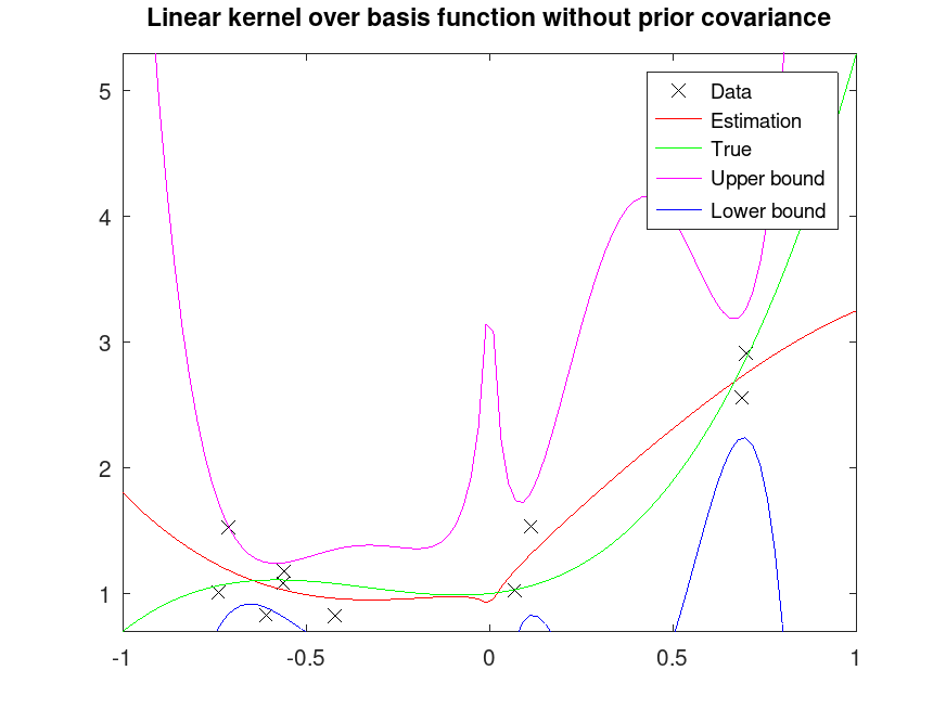
Example: 4
Projection over basis function with linear kernel
 pp = [2, 2, 0.3, 1];
 n = 10;
 rand ('seed', 145);
 X = 2 * rand (n, 1) - 1;
 randn ('seed', 45);
 Y = polyval (pp, X) + 0.3 * randn (n, 1);
Powers
px = [sqrt(abs(X)), X, X.^2, X.^3];
Points for interpolation/extrapolation
 Xfit = linspace (-1, 1, 100)';
 pxi = [sqrt(abs(Xfit)), Xfit, Xfit.^2, Xfit.^3];
Fit regression model without any assumption on prior covariance
[Yfit, Yint, Ysd] = regress_gp (px, Y, pxi);
Plot fitted data
 plot (X, Y, 'xk;Data;', Xfit, Yfit, 'r-;Estimation;', ...
                         Xfit, polyval (pp, Xfit), 'g-;True;');
 axis tight
 axis manual
 hold on
 plot (Xfit, Yint(:,1), 'm-;Upper bound;', Xfit, Yint(:,2), 'b-;Lower bound;');
 hold off
 title ('Linear kernel over basis function without prior covariance');
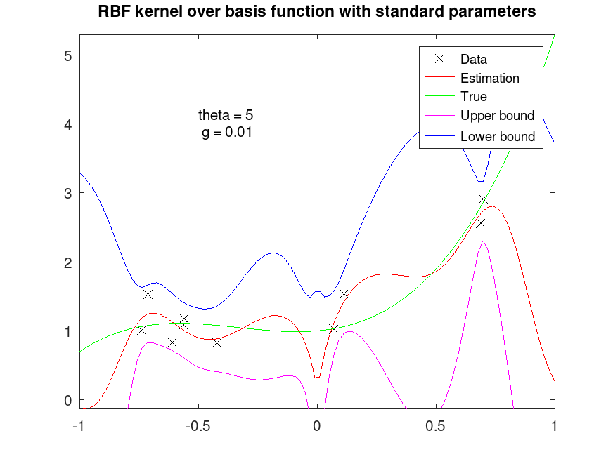
Example: 5
Projection over basis function with rbf kernel
 pp = [2, 2, 0.3, 1];
 n = 10;
 rand ('seed', 145);
 X = 2 * rand (n, 1) - 1;
 randn ('seed', 45);
 Y = polyval (pp, X) + 0.3 * randn (n, 1);
Powers
px = [sqrt(abs(X)), X, X.^2, X.^3];
Points for interpolation/extrapolation
 Xfit = linspace (-1, 1, 100)';
 pxi = [sqrt(abs(Xfit)), Xfit, Xfit.^2, Xfit.^3];
Fit regression model with RBF kernel (standard parameters)
[Yfit, Yint, Ysd] = regress_gp (px, Y, pxi, 'rbf');
Plot fitted data
 plot (X, Y, 'xk;Data;', Xfit, Yfit, 'r-;Estimation;', ...
                         Xfit, polyval (pp, Xfit), 'g-;True;');
 axis tight
 axis manual
 hold on
 plot (Xfit, Yint(:,1), 'm-;Upper bound;', Xfit, Yint(:,2), 'b-;Lower bound;');
 hold off
 title ('RBF kernel over basis function with standard parameters');
 text (-0.5, 4, "theta = 5\n g = 0.01");
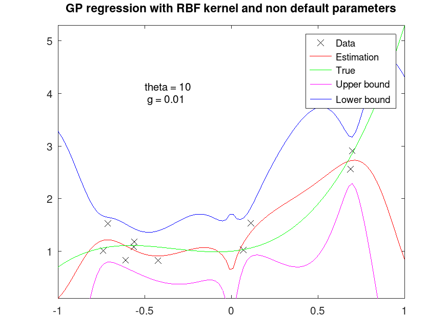
Example: 6
Projection over basis function with rbf kernel
 pp = [2, 2, 0.3, 1];
 n = 10;
 rand ('seed', 145);
 X = 2 * rand (n, 1) - 1;
 randn ('seed', 45);
 Y = polyval (pp, X) + 0.3 * randn (n, 1);
Powers
px = [sqrt(abs(X)), X, X.^2, X.^3];
Points for interpolation/extrapolation
 Xfit = linspace (-1, 1, 100)';
 pxi = [sqrt(abs(Xfit)), Xfit, Xfit.^2, Xfit.^3];
Fit regression model with RBF kernel with different parameters
[Yfit, Yint, Ysd] = regress_gp (px, Y, pxi, 'rbf', 10, 0.01);
Plot fitted data
 plot (X, Y, 'xk;Data;', Xfit, Yfit, 'r-;Estimation;', ...
                         Xfit, polyval (pp, Xfit), 'g-;True;');
 axis tight
 axis manual
 hold on
 plot (Xfit, Yint(:,1), 'm-;Upper bound;', Xfit, Yint(:,2), 'b-;Lower bound;');
 hold off
 title ('GP regression with RBF kernel and non default parameters');
 text (-0.5, 4, "theta = 10\n g = 0.01");
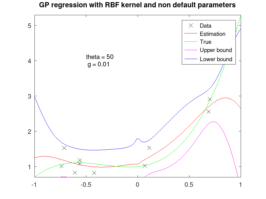
Fit regression model with RBF kernel with different parameters
[Yfit, Yint, Ysd] = regress_gp (px, Y, pxi, 'rbf', 50, 0.01);
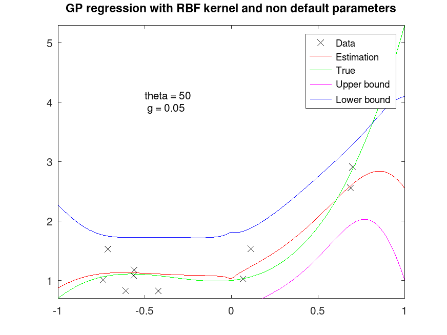
Plot fitted data
 figure
 plot (X, Y, 'xk;Data;', Xfit, Yfit, 'r-;Estimation;', ...
                         Xfit, polyval (pp, Xfit), 'g-;True;');
 axis tight
 axis manual
 hold on
 plot (Xfit, Yint(:,1), 'm-;Upper bound;', Xfit, Yint(:,2), 'b-;Lower bound;');
 hold off
 title ('GP regression with RBF kernel and non default parameters');
 text (-0.5, 4, "theta = 50\n g = 0.01");
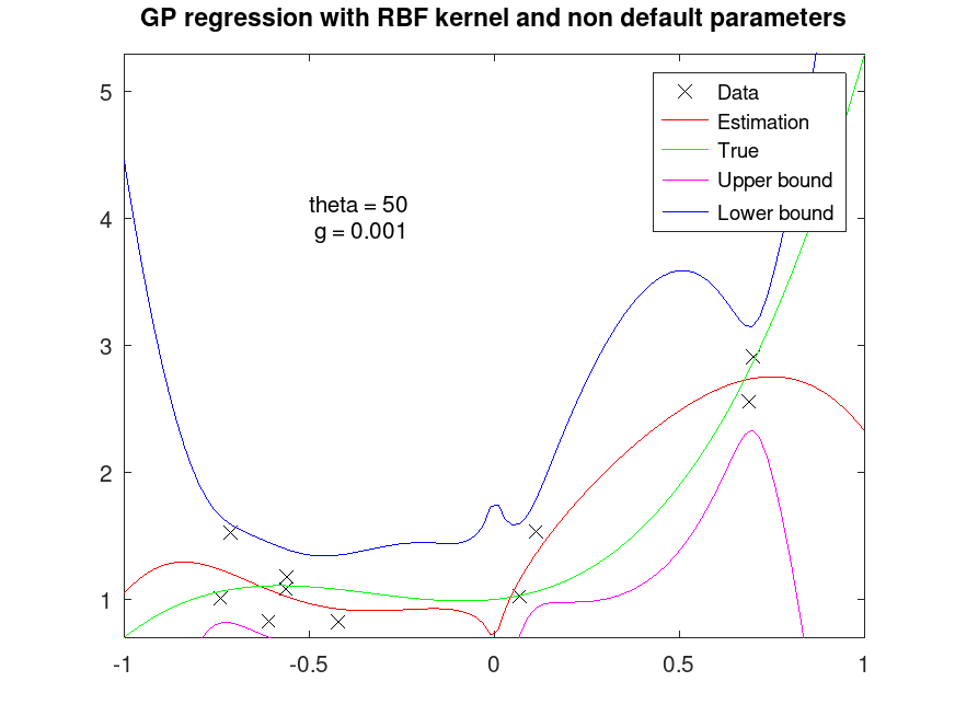
Fit regression model with RBF kernel with different parameters
[Yfit, Yint, Ysd] = regress_gp (px, Y, pxi, 'rbf', 50, 0.001);
Plot fitted data
 figure
 plot (X, Y, 'xk;Data;', Xfit, Yfit, 'r-;Estimation;', ...
                         Xfit, polyval (pp, Xfit), 'g-;True;');
 axis tight
 axis manual
 hold on
 plot (Xfit, Yint(:,1), 'm-;Upper bound;', Xfit, Yint(:,2), 'b-;Lower bound;');
 hold off
 title ('GP regression with RBF kernel and non default parameters');
 text (-0.5, 4, "theta = 50\n g = 0.001");
Fit regression model with RBF kernel with different parameters
[Yfit, Yint, Ysd] = regress_gp (px, Y, pxi, 'rbf', 50, 0.05);
Plot fitted data
 figure
 plot (X, Y, 'xk;Data;', Xfit, Yfit, 'r-;Estimation;', ...
                         Xfit, polyval (pp, Xfit), 'g-;True;');
 axis tight
 axis manual
 hold on
 plot (Xfit, Yint(:,1), 'm-;Upper bound;', Xfit, Yint(:,2), 'b-;Lower bound;');
 hold off
 title ('GP regression with RBF kernel and non default parameters');
 text (-0.5, 4, "theta = 50\n g = 0.05");
Example: 7
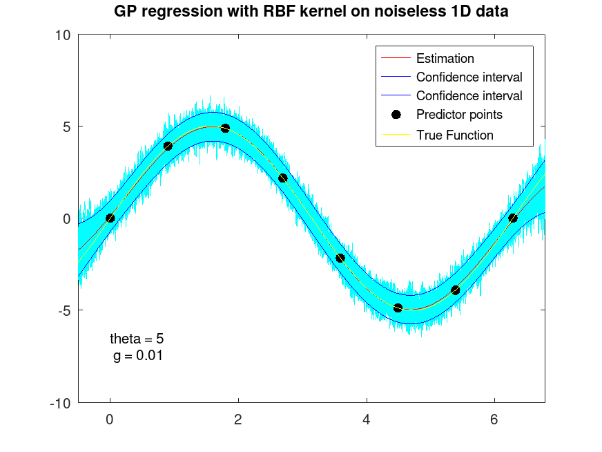
RBF fitting on noiseless 1D Data
 x = [0:2*pi/7:2*pi]';
 y = 5 * sin (x);
Predictive grid of 500 equally spaced locations
xi = [-0.5:(2*pi+1)/499:2*pi+0.5]';
Fit regression model with RBF kernel
[Yfit, Yint, Ysd] = regress_gp (x, y, xi, 'rbf');
Plot fitted data
 r = mvnrnd (Yfit, diag (Ysd)', 50);
 plot (xi, r', 'c-');
 hold on
 plot (xi, Yfit, 'r-;Estimation;', xi, Yint, 'b-;Confidence interval;');
 plot (x, y, '.k;Predictor points;', 'markersize', 20)
 plot (xi, 5 * sin (xi), '-y;True Function;');
 xlim ([-0.5,2*pi+0.5]);
 ylim ([-10,10]);
 hold off
 title ('GP regression with RBF kernel on noiseless 1D data');
 text (0, -7, "theta = 5\n g = 0.01");
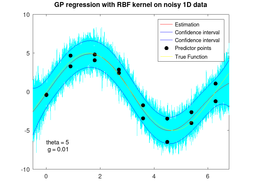
Example: 8
RBF fitting on noisy 1D Data
 x = [0:2*pi/7:2*pi]';
 x = [x; x];
 y = 5 * sin (x) + randn (size (x));
Predictive grid of 500 equally spaced locations
xi = [-0.5:(2*pi+1)/499:2*pi+0.5]';
Fit regression model with RBF kernel
[Yfit, Yint, Ysd] = regress_gp (x, y, xi, 'rbf');
Plot fitted data
 r = mvnrnd (Yfit, diag (Ysd)', 50);
 plot (xi, r', 'c-');
 hold on
 plot (xi, Yfit, 'r-;Estimation;', xi, Yint, 'b-;Confidence interval;');
 plot (x, y, '.k;Predictor points;', 'markersize', 20)
 plot (xi, 5 * sin (xi), '-y;True Function;');
 xlim ([-0.5,2*pi+0.5]);
 ylim ([-10,10]);
 hold off
 title ('GP regression with RBF kernel on noisy 1D data');
 text (0, -7, "theta = 5\n g = 0.01");