Categories &
Functions List
- BetaDistribution
- BinomialDistribution
- BirnbaumSaundersDistribution
- BurrDistribution
- ExponentialDistribution
- ExtremeValueDistribution
- GammaDistribution
- GeneralizedExtremeValueDistribution
- GeneralizedParetoDistribution
- HalfNormalDistribution
- InverseGaussianDistribution
- LogisticDistribution
- LoglogisticDistribution
- LognormalDistribution
- LoguniformDistribution
- MultinomialDistribution
- NakagamiDistribution
- NegativeBinomialDistribution
- NormalDistribution
- PiecewiseLinearDistribution
- PoissonDistribution
- RayleighDistribution
- RicianDistribution
- tLocationScaleDistribution
- TriangularDistribution
- UniformDistribution
- WeibullDistribution
- betafit
- betalike
- binofit
- binolike
- bisafit
- bisalike
- burrfit
- burrlike
- evfit
- evlike
- expfit
- explike
- gamfit
- gamlike
- geofit
- gevfit_lmom
- gevfit
- gevlike
- gpfit
- gplike
- gumbelfit
- gumbellike
- hnfit
- hnlike
- invgfit
- invglike
- logifit
- logilike
- loglfit
- logllike
- lognfit
- lognlike
- nakafit
- nakalike
- nbinfit
- nbinlike
- normfit
- normlike
- poissfit
- poisslike
- raylfit
- rayllike
- ricefit
- ricelike
- tlsfit
- tlslike
- unidfit
- unifit
- wblfit
- wbllike
- betacdf
- betainv
- betapdf
- betarnd
- binocdf
- binoinv
- binopdf
- binornd
- bisacdf
- bisainv
- bisapdf
- bisarnd
- burrcdf
- burrinv
- burrpdf
- burrrnd
- bvncdf
- bvtcdf
- cauchycdf
- cauchyinv
- cauchypdf
- cauchyrnd
- chi2cdf
- chi2inv
- chi2pdf
- chi2rnd
- copulacdf
- copulapdf
- copularnd
- evcdf
- evinv
- evpdf
- evrnd
- expcdf
- expinv
- exppdf
- exprnd
- fcdf
- finv
- fpdf
- frnd
- gamcdf
- gaminv
- gampdf
- gamrnd
- geocdf
- geoinv
- geopdf
- geornd
- gevcdf
- gevinv
- gevpdf
- gevrnd
- gpcdf
- gpinv
- gppdf
- gprnd
- gumbelcdf
- gumbelinv
- gumbelpdf
- gumbelrnd
- hncdf
- hninv
- hnpdf
- hnrnd
- hygecdf
- hygeinv
- hygepdf
- hygernd
- invgcdf
- invginv
- invgpdf
- invgrnd
- iwishpdf
- iwishrnd
- jsucdf
- jsupdf
- laplacecdf
- laplaceinv
- laplacepdf
- laplacernd
- logicdf
- logiinv
- logipdf
- logirnd
- loglcdf
- loglinv
- loglpdf
- loglrnd
- logncdf
- logninv
- lognpdf
- lognrnd
- mnpdf
- mnrnd
- mvncdf
- mvnpdf
- mvnrnd
- mvtcdf
- mvtpdf
- mvtrnd
- mvtcdfqmc
- nakacdf
- nakainv
- nakapdf
- nakarnd
- nbincdf
- nbininv
- nbinpdf
- nbinrnd
- ncfcdf
- ncfinv
- ncfpdf
- ncfrnd
- nctcdf
- nctinv
- nctpdf
- nctrnd
- ncx2cdf
- ncx2inv
- ncx2pdf
- ncx2rnd
- normcdf
- norminv
- normpdf
- normrnd
- plcdf
- plinv
- plpdf
- plrnd
- poisscdf
- poissinv
- poisspdf
- poissrnd
- raylcdf
- raylinv
- raylpdf
- raylrnd
- ricecdf
- riceinv
- ricepdf
- ricernd
- tcdf
- tinv
- tpdf
- trnd
- tlscdf
- tlsinv
- tlspdf
- tlsrnd
- tricdf
- triinv
- tripdf
- trirnd
- unidcdf
- unidinv
- unidpdf
- unidrnd
- unifcdf
- unifinv
- unifpdf
- unifrnd
- vmcdf
- vminv
- vmpdf
- vmrnd
- wblcdf
- wblinv
- wblpdf
- wblrnd
- wienrnd
- wishpdf
- wishrnd
- adtest
- anova
- anova1
- anova2
- anovan
- bartlett_test
- barttest
- binotest
- chi2gof
- chi2test
- correlation_test
- fishertest
- friedman
- hotelling_t2test
- hotelling_t2test2
- kruskalwallis
- kstest
- kstest2
- levene_test
- manova1
- mcnemar_test
- multcompare
- ranksum
- regression_ftest
- regression_ttest
- runstest
- sampsizepwr
- signrank
- signtest
- tiedrank
- ttest
- ttest2
- vartest
- vartest2
- vartestn
- ztest
- ztest2
Function Reference: binofit
statistics: pshat = binofit (x, n)
statistics: [pshat, psci] = binofit (x, n)
statistics: [pshat, psci] = binofit (x, n, alpha)
Estimate parameter and confidence intervals for the binomial distribution.
pshat = binofit (x, n) returns the maximum
likelihood estimate (MLE) of the probability of success for the binomial
distribution. x and n are scalars containing the number of
successes and the number of trials, respectively. If x and n are
vectors, binofit returns a vector of estimates whose -th
element is the parameter estimate for x(i) and n(i). A scalar
value for x or n is expanded to the same size as the other input.
[pshat, psci] = binofit (x, n, alpha)
also returns the 100 * (1 - alpha) percent confidence intervals
of the estimated parameter. By default, the optional argument alpha
is 0.05 corresponding to 95% confidence intervals.
binofit treats a vector x as a collection of measurements from
separate samples, and returns a vector of estimates. If you want to treat
x as a single sample and compute a single parameter estimate and
confidence interval, use binofit (sum (x), sum (n)) when
n is a vector, and
binofit (sum (x), n * length (x)) when n is a
scalar.
Further information about the binomial distribution can be found at https://en.wikipedia.org/wiki/Binomial_distribution
See also: binocdf, binoinv, binopdf, binornd, binolike, binostat
Source Code: binofit
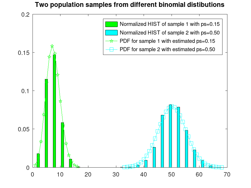
Example: 1
Sample 2 populations from different binomial distributions
 rand ('seed', 1);    # for reproducibility
 r1 = binornd (50, 0.15, 1000, 1);
 rand ('seed', 2);    # for reproducibility
 r2 = binornd (100, 0.5, 1000, 1);
 r = [r1, r2];
Plot them normalized and fix their colors
 hist (r, 23, 0.35);
 h = findobj (gca, 'Type', 'patch');
 set (h(1), 'facecolor', 'c');
 set (h(2), 'facecolor', 'g');
 hold on
Estimate their probability of success
 pshatA = binofit (r(:,1), 50);
 pshatB = binofit (r(:,2), 100);
Plot their estimated PDFs
 x = [min(r(:,1)):max(r(:,1))];
 y = binopdf (x, 50, mean (pshatA));
 plot (x, y, '-pg');
 x = [min(r(:,2)):max(r(:,2))];
 y = binopdf (x, 100, mean (pshatB));
 plot (x, y, '-sc');
 ylim ([0, 0.2])
 legend ({'Normalized HIST of sample 1 with ps=0.15', ...
          'Normalized HIST of sample 2 with ps=0.50', ...
          sprintf("PDF for sample 1 with estimated ps=%0.2f", ...
                  mean (pshatA)), ...
          sprintf("PDF for sample 2 with estimated ps=%0.2f", ...
                  mean (pshatB))})
 title ('Two population samples from different binomial distributions')
 hold off