Categories &
Functions List
- BetaDistribution
- BinomialDistribution
- BirnbaumSaundersDistribution
- BurrDistribution
- ExponentialDistribution
- ExtremeValueDistribution
- GammaDistribution
- GeneralizedExtremeValueDistribution
- GeneralizedParetoDistribution
- HalfNormalDistribution
- InverseGaussianDistribution
- LogisticDistribution
- LoglogisticDistribution
- LognormalDistribution
- LoguniformDistribution
- MultinomialDistribution
- NakagamiDistribution
- NegativeBinomialDistribution
- NormalDistribution
- PiecewiseLinearDistribution
- PoissonDistribution
- RayleighDistribution
- RicianDistribution
- tLocationScaleDistribution
- TriangularDistribution
- UniformDistribution
- WeibullDistribution
- betafit
- betalike
- binofit
- binolike
- bisafit
- bisalike
- burrfit
- burrlike
- evfit
- evlike
- expfit
- explike
- gamfit
- gamlike
- geofit
- gevfit_lmom
- gevfit
- gevlike
- gpfit
- gplike
- gumbelfit
- gumbellike
- hnfit
- hnlike
- invgfit
- invglike
- logifit
- logilike
- loglfit
- logllike
- lognfit
- lognlike
- nakafit
- nakalike
- nbinfit
- nbinlike
- normfit
- normlike
- poissfit
- poisslike
- raylfit
- rayllike
- ricefit
- ricelike
- tlsfit
- tlslike
- unidfit
- unifit
- wblfit
- wbllike
- betacdf
- betainv
- betapdf
- betarnd
- binocdf
- binoinv
- binopdf
- binornd
- bisacdf
- bisainv
- bisapdf
- bisarnd
- burrcdf
- burrinv
- burrpdf
- burrrnd
- bvncdf
- bvtcdf
- cauchycdf
- cauchyinv
- cauchypdf
- cauchyrnd
- chi2cdf
- chi2inv
- chi2pdf
- chi2rnd
- copulacdf
- copulapdf
- copularnd
- evcdf
- evinv
- evpdf
- evrnd
- expcdf
- expinv
- exppdf
- exprnd
- fcdf
- finv
- fpdf
- frnd
- gamcdf
- gaminv
- gampdf
- gamrnd
- geocdf
- geoinv
- geopdf
- geornd
- gevcdf
- gevinv
- gevpdf
- gevrnd
- gpcdf
- gpinv
- gppdf
- gprnd
- gumbelcdf
- gumbelinv
- gumbelpdf
- gumbelrnd
- hncdf
- hninv
- hnpdf
- hnrnd
- hygecdf
- hygeinv
- hygepdf
- hygernd
- invgcdf
- invginv
- invgpdf
- invgrnd
- iwishpdf
- iwishrnd
- jsucdf
- jsupdf
- laplacecdf
- laplaceinv
- laplacepdf
- laplacernd
- logicdf
- logiinv
- logipdf
- logirnd
- loglcdf
- loglinv
- loglpdf
- loglrnd
- logncdf
- logninv
- lognpdf
- lognrnd
- mnpdf
- mnrnd
- mvncdf
- mvnpdf
- mvnrnd
- mvtcdf
- mvtpdf
- mvtrnd
- mvtcdfqmc
- nakacdf
- nakainv
- nakapdf
- nakarnd
- nbincdf
- nbininv
- nbinpdf
- nbinrnd
- ncfcdf
- ncfinv
- ncfpdf
- ncfrnd
- nctcdf
- nctinv
- nctpdf
- nctrnd
- ncx2cdf
- ncx2inv
- ncx2pdf
- ncx2rnd
- normcdf
- norminv
- normpdf
- normrnd
- plcdf
- plinv
- plpdf
- plrnd
- poisscdf
- poissinv
- poisspdf
- poissrnd
- raylcdf
- raylinv
- raylpdf
- raylrnd
- ricecdf
- riceinv
- ricepdf
- ricernd
- tcdf
- tinv
- tpdf
- trnd
- tlscdf
- tlsinv
- tlspdf
- tlsrnd
- tricdf
- triinv
- tripdf
- trirnd
- unidcdf
- unidinv
- unidpdf
- unidrnd
- unifcdf
- unifinv
- unifpdf
- unifrnd
- vmcdf
- vminv
- vmpdf
- vmrnd
- wblcdf
- wblinv
- wblpdf
- wblrnd
- wienrnd
- wishpdf
- wishrnd
- adtest
- anova
- anova1
- anova2
- anovan
- bartlett_test
- barttest
- binotest
- chi2gof
- chi2test
- correlation_test
- fishertest
- friedman
- hotelling_t2test
- hotelling_t2test2
- kruskalwallis
- kstest
- kstest2
- levene_test
- manova1
- mcnemar_test
- multcompare
- ranksum
- regression_ftest
- regression_ttest
- runstest
- sampsizepwr
- signrank
- signtest
- tiedrank
- ttest
- ttest2
- vartest
- vartest2
- vartestn
- ztest
- ztest2
Function Reference: normcdf
statistics: p = normcdf (x)
statistics: p = normcdf (x, mu)
statistics: p = normcdf (x, mu, sigma)
statistics: p = normcdf (…,
'upper')statistics: [p, plo, pup] = normcdf (x, mu, sigma, pcov)
statistics: [p, plo, pup] = normcdf (x, mu, sigma, pcov, alpha)
statistics: [p, plo, pup] = normcdf (…,
'upper')
Normal cumulative distribution function (CDF).
For each element of x, compute the cumulative distribution function (CDF) of the normal distribution with mean mu and standard deviation sigma. The size of p is the common size of x, mu and sigma. A scalar input functions as a constant matrix of the same size as the other inputs.
Default values are mu = 0, sigma = 1.
When called with three output arguments, i.e. [p, plo,
pup], normcdf computes the confidence bounds for p when
the input parameters mu and sigma are estimates. In such case,
pcov, a matrix containing the covariance matrix of the
estimated parameters, is necessary. Optionally, alpha, which has a
default value of 0.05, specifies the 100 * (1 - alpha) percent
confidence bounds. plo and pup are arrays of the same size as
p containing the lower and upper confidence bounds.
[…] = normcdf (…, "upper") computes the upper tail
probability of the normal distribution with parameters mu and
sigma, at the values in x. This can be used to compute a
right-tailed p-value. To compute a two-tailed p-value, use
2 * normcdf (-abs (x), mu, sigma).
Further information about the normal distribution can be found at https://en.wikipedia.org/wiki/Normal_distribution
See also: norminv, normpdf, normrnd, normfit, normlike, normstat
Source Code: normcdf
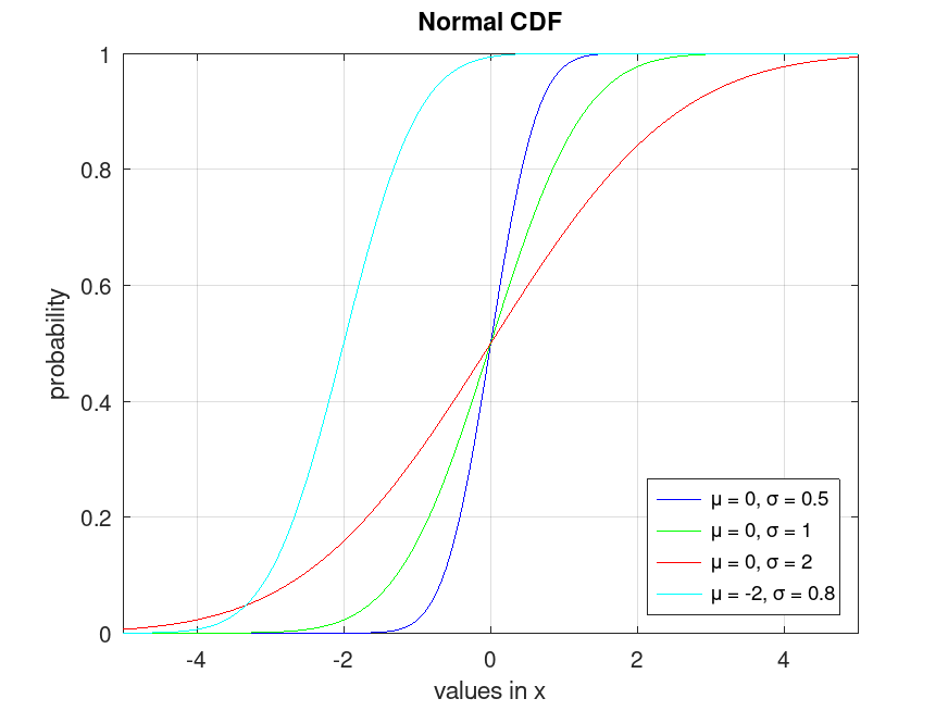
Example: 1
Plot various CDFs from the normal distribution
 x = -5:0.01:5;
 p1 = normcdf (x, 0, 0.5);
 p2 = normcdf (x, 0, 1);
 p3 = normcdf (x, 0, 2);
 p4 = normcdf (x, -2, 0.8);
 plot (x, p1, '-b', x, p2, '-g', x, p3, '-r', x, p4, '-c')
 grid on
 xlim ([-5, 5])
 legend ({'μ = 0, σ = 0.5', 'μ = 0, σ = 1', ...
          'μ = 0, σ = 2', 'μ = -2, σ = 0.8'}, 'location', 'southeast')
 title ('Normal CDF')
 xlabel ('values in x')
 ylabel ('probability')