Categories &
Functions List
- BetaDistribution
- BinomialDistribution
- BirnbaumSaundersDistribution
- BurrDistribution
- ExponentialDistribution
- ExtremeValueDistribution
- GammaDistribution
- GeneralizedExtremeValueDistribution
- GeneralizedParetoDistribution
- HalfNormalDistribution
- InverseGaussianDistribution
- LogisticDistribution
- LoglogisticDistribution
- LognormalDistribution
- LoguniformDistribution
- MultinomialDistribution
- NakagamiDistribution
- NegativeBinomialDistribution
- NormalDistribution
- PiecewiseLinearDistribution
- PoissonDistribution
- RayleighDistribution
- RicianDistribution
- tLocationScaleDistribution
- TriangularDistribution
- UniformDistribution
- WeibullDistribution
- betafit
- betalike
- binofit
- binolike
- bisafit
- bisalike
- burrfit
- burrlike
- evfit
- evlike
- expfit
- explike
- gamfit
- gamlike
- geofit
- gevfit_lmom
- gevfit
- gevlike
- gpfit
- gplike
- gumbelfit
- gumbellike
- hnfit
- hnlike
- invgfit
- invglike
- logifit
- logilike
- loglfit
- logllike
- lognfit
- lognlike
- nakafit
- nakalike
- nbinfit
- nbinlike
- normfit
- normlike
- poissfit
- poisslike
- raylfit
- rayllike
- ricefit
- ricelike
- tlsfit
- tlslike
- unidfit
- unifit
- wblfit
- wbllike
- betacdf
- betainv
- betapdf
- betarnd
- binocdf
- binoinv
- binopdf
- binornd
- bisacdf
- bisainv
- bisapdf
- bisarnd
- burrcdf
- burrinv
- burrpdf
- burrrnd
- bvncdf
- bvtcdf
- cauchycdf
- cauchyinv
- cauchypdf
- cauchyrnd
- chi2cdf
- chi2inv
- chi2pdf
- chi2rnd
- copulacdf
- copulapdf
- copularnd
- evcdf
- evinv
- evpdf
- evrnd
- expcdf
- expinv
- exppdf
- exprnd
- fcdf
- finv
- fpdf
- frnd
- gamcdf
- gaminv
- gampdf
- gamrnd
- geocdf
- geoinv
- geopdf
- geornd
- gevcdf
- gevinv
- gevpdf
- gevrnd
- gpcdf
- gpinv
- gppdf
- gprnd
- gumbelcdf
- gumbelinv
- gumbelpdf
- gumbelrnd
- hncdf
- hninv
- hnpdf
- hnrnd
- hygecdf
- hygeinv
- hygepdf
- hygernd
- invgcdf
- invginv
- invgpdf
- invgrnd
- iwishpdf
- iwishrnd
- jsucdf
- jsupdf
- laplacecdf
- laplaceinv
- laplacepdf
- laplacernd
- logicdf
- logiinv
- logipdf
- logirnd
- loglcdf
- loglinv
- loglpdf
- loglrnd
- logncdf
- logninv
- lognpdf
- lognrnd
- mnpdf
- mnrnd
- mvncdf
- mvnpdf
- mvnrnd
- mvtcdf
- mvtpdf
- mvtrnd
- mvtcdfqmc
- nakacdf
- nakainv
- nakapdf
- nakarnd
- nbincdf
- nbininv
- nbinpdf
- nbinrnd
- ncfcdf
- ncfinv
- ncfpdf
- ncfrnd
- nctcdf
- nctinv
- nctpdf
- nctrnd
- ncx2cdf
- ncx2inv
- ncx2pdf
- ncx2rnd
- normcdf
- norminv
- normpdf
- normrnd
- plcdf
- plinv
- plpdf
- plrnd
- poisscdf
- poissinv
- poisspdf
- poissrnd
- raylcdf
- raylinv
- raylpdf
- raylrnd
- ricecdf
- riceinv
- ricepdf
- ricernd
- tcdf
- tinv
- tpdf
- trnd
- tlscdf
- tlsinv
- tlspdf
- tlsrnd
- tricdf
- triinv
- tripdf
- trirnd
- unidcdf
- unidinv
- unidpdf
- unidrnd
- unifcdf
- unifinv
- unifpdf
- unifrnd
- vmcdf
- vminv
- vmpdf
- vmrnd
- wblcdf
- wblinv
- wblpdf
- wblrnd
- wienrnd
- wishpdf
- wishrnd
- adtest
- anova
- anova1
- anova2
- anovan
- bartlett_test
- barttest
- binotest
- chi2gof
- chi2test
- correlation_test
- fishertest
- friedman
- hotelling_t2test
- hotelling_t2test2
- kruskalwallis
- kstest
- kstest2
- levene_test
- manova1
- mcnemar_test
- multcompare
- ranksum
- regression_ftest
- regression_ttest
- runstest
- sampsizepwr
- signrank
- signtest
- tiedrank
- ttest
- ttest2
- vartest
- vartest2
- vartestn
- ztest
- ztest2
Function Reference: gumbelfit
statistics: paramhat = gumbelfit (x)
statistics: [paramhat, paramci] = gumbelfit (x)
statistics: [paramhat, paramci] = gumbelfit (x, alpha)
statistics: […] = gumbelfit (x, alpha, censor)
statistics: […] = gumbelfit (x, alpha, censor, freq)
statistics: […] = gumbelfit (x, alpha, censor, freq, options)
Estimate parameters and confidence intervals for Gumbel distribution.
paramhat = gumbelfit (x) returns the maximum likelihood
estimates of the parameters of the Gumbel distribution (also known as
the extreme value or the type I generalized extreme value distribution) given
in x. paramhat(1) is the location parameter, mu,
and paramhat(2) is the scale parameter, beta.
[paramhat, paramci] = gumbelfit (x) returns the 95%
confidence intervals for the parameter estimates.
[…] = gumbelfit (x, alpha) also returns the
100 * (1 - alpha) percent confidence intervals for the
parameter estimates. By default, the optional argument alpha is
0.05 corresponding to 95% confidence intervals. Pass in [] for
alpha to use the default values.
[…] = gumbelfit (x, alpha, censor) accepts a
boolean vector, censor, of the same size as x with 1s for
observations that are right-censored and 0s for observations that are
observed exactly. By default, or if left empty,
censor = zeros (size (x)).
[…] = gumbelfit (x, alpha, censor, freq)
accepts a frequency vector, freq, of the same size as x.
freq typically contains integer frequencies for the corresponding
elements in x, but it can contain any non-integer non-negative values.
By default, or if left empty, freq = ones (size (x)).
[…] = gumbelfit (…, options) specifies control
parameters for the iterative algorithm used to compute the maximum likelihood
estimates. options is a structure with the following field and its
default value:
-
options.Display = "off" -
options.MaxFunEvals = 400 -
options.MaxIter = 200 -
options.TolX = 1e-6
The Gumbel distribution is used to model the distribution of the maximum (or
the minimum) of a number of samples of various distributions. This version
is suitable for modeling maxima. For modeling minima, use the alternative
extreme value fitting function, evfit.
Further information about the Gumbel distribution can be found at https://en.wikipedia.org/wiki/Gumbel_distribution
See also: gumbelcdf, gumbelinv, gumbelpdf, gumbelrnd, gumbellike, gumbelstat, evfit
Source Code: gumbelfit
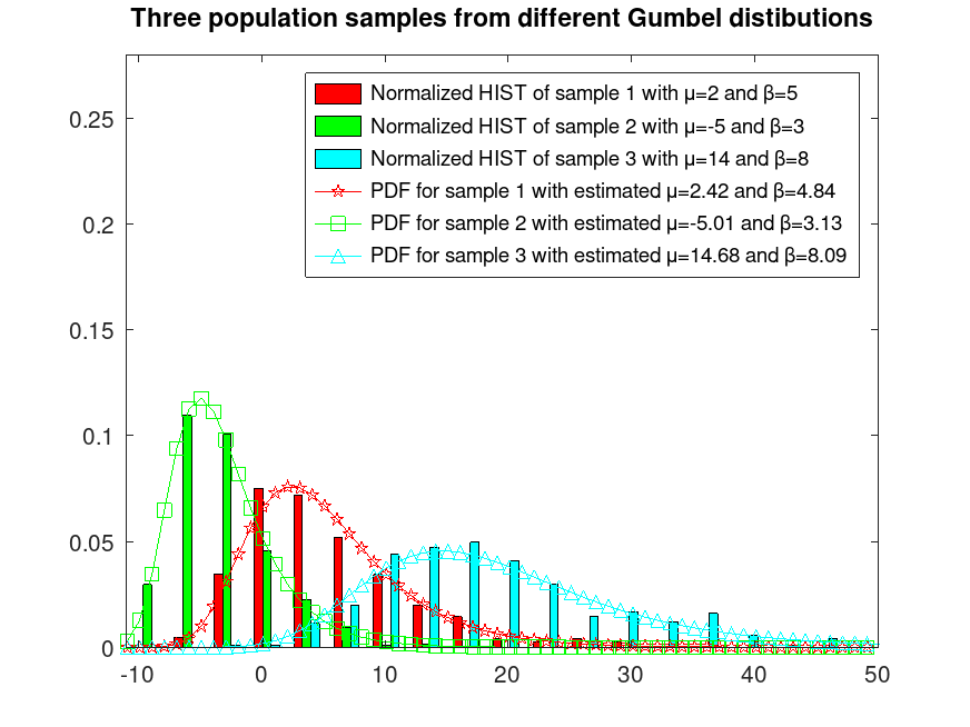
Example: 1
Sample 3 populations from different Gumbel distributions
 rand ('seed', 1);    # for reproducibility
 r1 = gumbelrnd (2, 5, 400, 1);
 rand ('seed', 11);    # for reproducibility
 r2 = gumbelrnd (-5, 3, 400, 1);
 rand ('seed', 16);    # for reproducibility
 r3 = gumbelrnd (14, 8, 400, 1);
 r = [r1, r2, r3];
Plot them normalized and fix their colors
 hist (r, 25, 0.32);
 h = findobj (gca, 'Type', 'patch');
 set (h(1), 'facecolor', 'c');
 set (h(2), 'facecolor', 'g');
 set (h(3), 'facecolor', 'r');
 ylim ([0, 0.28])
 xlim ([-11, 50]);
 hold on
Estimate their MU and BETA parameters
 mu_betaA = gumbelfit (r(:,1));
 mu_betaB = gumbelfit (r(:,2));
 mu_betaC = gumbelfit (r(:,3));
Plot their estimated PDFs
 x = [min(r(:)):max(r(:))];
 y = gumbelpdf (x, mu_betaA(1), mu_betaA(2));
 plot (x, y, '-pr');
 y = gumbelpdf (x, mu_betaB(1), mu_betaB(2));
 plot (x, y, '-sg');
 y = gumbelpdf (x, mu_betaC(1), mu_betaC(2));
 plot (x, y, '-^c');
 legend ({'Normalized HIST of sample 1 with μ=2 and β=5', ...
          'Normalized HIST of sample 2 with μ=-5 and β=3', ...
          'Normalized HIST of sample 3 with μ=14 and β=8', ...
          sprintf("PDF for sample 1 with estimated μ=%0.2f and β=%0.2f", ...
                  mu_betaA(1), mu_betaA(2)), ...
          sprintf("PDF for sample 2 with estimated μ=%0.2f and β=%0.2f", ...
                  mu_betaB(1), mu_betaB(2)), ...
          sprintf("PDF for sample 3 with estimated μ=%0.2f and β=%0.2f", ...
                  mu_betaC(1), mu_betaC(2))})
 title ('Three population samples from different Gumbel distributions')
 hold off