Categories &
Functions List
- BetaDistribution
- BinomialDistribution
- BirnbaumSaundersDistribution
- BurrDistribution
- ExponentialDistribution
- ExtremeValueDistribution
- GammaDistribution
- GeneralizedExtremeValueDistribution
- GeneralizedParetoDistribution
- HalfNormalDistribution
- InverseGaussianDistribution
- LogisticDistribution
- LoglogisticDistribution
- LognormalDistribution
- LoguniformDistribution
- MultinomialDistribution
- NakagamiDistribution
- NegativeBinomialDistribution
- NormalDistribution
- PiecewiseLinearDistribution
- PoissonDistribution
- RayleighDistribution
- RicianDistribution
- tLocationScaleDistribution
- TriangularDistribution
- UniformDistribution
- WeibullDistribution
- betafit
- betalike
- binofit
- binolike
- bisafit
- bisalike
- burrfit
- burrlike
- evfit
- evlike
- expfit
- explike
- gamfit
- gamlike
- geofit
- gevfit_lmom
- gevfit
- gevlike
- gpfit
- gplike
- gumbelfit
- gumbellike
- hnfit
- hnlike
- invgfit
- invglike
- logifit
- logilike
- loglfit
- logllike
- lognfit
- lognlike
- nakafit
- nakalike
- nbinfit
- nbinlike
- normfit
- normlike
- poissfit
- poisslike
- raylfit
- rayllike
- ricefit
- ricelike
- tlsfit
- tlslike
- unidfit
- unifit
- wblfit
- wbllike
- betacdf
- betainv
- betapdf
- betarnd
- binocdf
- binoinv
- binopdf
- binornd
- bisacdf
- bisainv
- bisapdf
- bisarnd
- burrcdf
- burrinv
- burrpdf
- burrrnd
- bvncdf
- bvtcdf
- cauchycdf
- cauchyinv
- cauchypdf
- cauchyrnd
- chi2cdf
- chi2inv
- chi2pdf
- chi2rnd
- copulacdf
- copulapdf
- copularnd
- evcdf
- evinv
- evpdf
- evrnd
- expcdf
- expinv
- exppdf
- exprnd
- fcdf
- finv
- fpdf
- frnd
- gamcdf
- gaminv
- gampdf
- gamrnd
- geocdf
- geoinv
- geopdf
- geornd
- gevcdf
- gevinv
- gevpdf
- gevrnd
- gpcdf
- gpinv
- gppdf
- gprnd
- gumbelcdf
- gumbelinv
- gumbelpdf
- gumbelrnd
- hncdf
- hninv
- hnpdf
- hnrnd
- hygecdf
- hygeinv
- hygepdf
- hygernd
- invgcdf
- invginv
- invgpdf
- invgrnd
- iwishpdf
- iwishrnd
- jsucdf
- jsupdf
- laplacecdf
- laplaceinv
- laplacepdf
- laplacernd
- logicdf
- logiinv
- logipdf
- logirnd
- loglcdf
- loglinv
- loglpdf
- loglrnd
- logncdf
- logninv
- lognpdf
- lognrnd
- mnpdf
- mnrnd
- mvncdf
- mvnpdf
- mvnrnd
- mvtcdf
- mvtpdf
- mvtrnd
- mvtcdfqmc
- nakacdf
- nakainv
- nakapdf
- nakarnd
- nbincdf
- nbininv
- nbinpdf
- nbinrnd
- ncfcdf
- ncfinv
- ncfpdf
- ncfrnd
- nctcdf
- nctinv
- nctpdf
- nctrnd
- ncx2cdf
- ncx2inv
- ncx2pdf
- ncx2rnd
- normcdf
- norminv
- normpdf
- normrnd
- plcdf
- plinv
- plpdf
- plrnd
- poisscdf
- poissinv
- poisspdf
- poissrnd
- raylcdf
- raylinv
- raylpdf
- raylrnd
- ricecdf
- riceinv
- ricepdf
- ricernd
- tcdf
- tinv
- tpdf
- trnd
- tlscdf
- tlsinv
- tlspdf
- tlsrnd
- tricdf
- triinv
- tripdf
- trirnd
- unidcdf
- unidinv
- unidpdf
- unidrnd
- unifcdf
- unifinv
- unifpdf
- unifrnd
- vmcdf
- vminv
- vmpdf
- vmrnd
- wblcdf
- wblinv
- wblpdf
- wblrnd
- wienrnd
- wishpdf
- wishrnd
- adtest
- anova
- anova1
- anova2
- anovan
- bartlett_test
- barttest
- binotest
- chi2gof
- chi2test
- correlation_test
- fishertest
- friedman
- hotelling_t2test
- hotelling_t2test2
- kruskalwallis
- kstest
- kstest2
- levene_test
- manova1
- mcnemar_test
- multcompare
- ranksum
- regression_ftest
- regression_ttest
- runstest
- sampsizepwr
- signrank
- signtest
- tiedrank
- ttest
- ttest2
- vartest
- vartest2
- vartestn
- ztest
- ztest2
Function Reference: ncfinv
statistics: x = ncfinv (p, df1, df2, lambda)
Inverse of the noncentral -cumulative distribution function (iCDF).
For each element of p, compute the quantile (the inverse of the CDF) of the noncentral -distribution with df1 and df2 degrees of freedom and noncentrality parameter lambda. The size of x is the common size of p, df1, df2, and lambda. A scalar input functions as a constant matrix of the same size as the other inputs.
ncfinv uses Newton’s method to converge to the solution.
Further information about the noncentral -distribution can be found at https://en.wikipedia.org/wiki/Noncentral_F-distribution
See also: ncfcdf, ncfpdf, ncfrnd, ncfstat, finv
Source Code: ncfinv
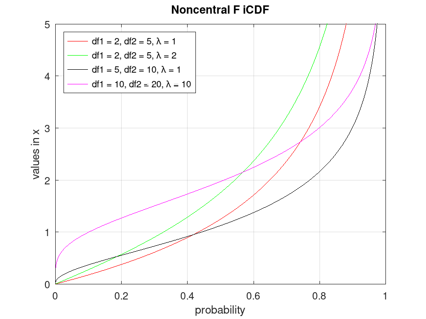
Example: 1
Plot various iCDFs from the noncentral F distribution
 p = 0.001:0.001:0.999;
 x1 = ncfinv (p, 2, 5, 1);
 x2 = ncfinv (p, 2, 5, 2);
 x3 = ncfinv (p, 5, 10, 1);
 x4 = ncfinv (p, 10, 20, 10);
 plot (p, x1, '-r', p, x2, '-g', p, x3, '-k', p, x4, '-m')
 grid on
 ylim ([0, 5])
 legend ({'df1 = 2, df2 = 5, λ = 1', 'df1 = 2, df2 = 5, λ = 2', ...
          'df1 = 5, df2 = 10, λ = 1', 'df1 = 10, df2 = 20, λ = 10'}, ...
         'location', 'northwest')
 title ('Noncentral F iCDF')
 xlabel ('probability')
 ylabel ('values in x')
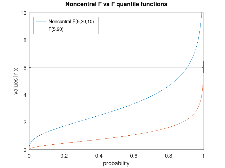
Example: 2
Compare the noncentral F iCDF with LAMBDA = 10 to the F iCDF with the same number of numerator and denominator degrees of freedom (5, 20)
 p = 0.001:0.001:0.999;
 x1 = ncfinv (p, 5, 20, 10);
 x2 = finv (p, 5, 20);
 plot (p, x1, '-', p, x2, '-');
 grid on
 ylim ([0, 10])
 legend ({'Noncentral F(5,20,10)', 'F(5,20)'}, 'location', 'northwest')
 title ('Noncentral F vs F quantile functions')
 xlabel ('probability')
 ylabel ('values in x')