Categories &
Functions List
- BetaDistribution
- BinomialDistribution
- BirnbaumSaundersDistribution
- BurrDistribution
- ExponentialDistribution
- ExtremeValueDistribution
- GammaDistribution
- GeneralizedExtremeValueDistribution
- GeneralizedParetoDistribution
- HalfNormalDistribution
- InverseGaussianDistribution
- LogisticDistribution
- LoglogisticDistribution
- LognormalDistribution
- LoguniformDistribution
- MultinomialDistribution
- NakagamiDistribution
- NegativeBinomialDistribution
- NormalDistribution
- PiecewiseLinearDistribution
- PoissonDistribution
- RayleighDistribution
- RicianDistribution
- tLocationScaleDistribution
- TriangularDistribution
- UniformDistribution
- WeibullDistribution
- betafit
- betalike
- binofit
- binolike
- bisafit
- bisalike
- burrfit
- burrlike
- evfit
- evlike
- expfit
- explike
- gamfit
- gamlike
- geofit
- gevfit_lmom
- gevfit
- gevlike
- gpfit
- gplike
- gumbelfit
- gumbellike
- hnfit
- hnlike
- invgfit
- invglike
- logifit
- logilike
- loglfit
- logllike
- lognfit
- lognlike
- nakafit
- nakalike
- nbinfit
- nbinlike
- normfit
- normlike
- poissfit
- poisslike
- raylfit
- rayllike
- ricefit
- ricelike
- tlsfit
- tlslike
- unidfit
- unifit
- wblfit
- wbllike
- betacdf
- betainv
- betapdf
- betarnd
- binocdf
- binoinv
- binopdf
- binornd
- bisacdf
- bisainv
- bisapdf
- bisarnd
- burrcdf
- burrinv
- burrpdf
- burrrnd
- bvncdf
- bvtcdf
- cauchycdf
- cauchyinv
- cauchypdf
- cauchyrnd
- chi2cdf
- chi2inv
- chi2pdf
- chi2rnd
- copulacdf
- copulapdf
- copularnd
- evcdf
- evinv
- evpdf
- evrnd
- expcdf
- expinv
- exppdf
- exprnd
- fcdf
- finv
- fpdf
- frnd
- gamcdf
- gaminv
- gampdf
- gamrnd
- geocdf
- geoinv
- geopdf
- geornd
- gevcdf
- gevinv
- gevpdf
- gevrnd
- gpcdf
- gpinv
- gppdf
- gprnd
- gumbelcdf
- gumbelinv
- gumbelpdf
- gumbelrnd
- hncdf
- hninv
- hnpdf
- hnrnd
- hygecdf
- hygeinv
- hygepdf
- hygernd
- invgcdf
- invginv
- invgpdf
- invgrnd
- iwishpdf
- iwishrnd
- jsucdf
- jsupdf
- laplacecdf
- laplaceinv
- laplacepdf
- laplacernd
- logicdf
- logiinv
- logipdf
- logirnd
- loglcdf
- loglinv
- loglpdf
- loglrnd
- logncdf
- logninv
- lognpdf
- lognrnd
- mnpdf
- mnrnd
- mvncdf
- mvnpdf
- mvnrnd
- mvtcdf
- mvtpdf
- mvtrnd
- mvtcdfqmc
- nakacdf
- nakainv
- nakapdf
- nakarnd
- nbincdf
- nbininv
- nbinpdf
- nbinrnd
- ncfcdf
- ncfinv
- ncfpdf
- ncfrnd
- nctcdf
- nctinv
- nctpdf
- nctrnd
- ncx2cdf
- ncx2inv
- ncx2pdf
- ncx2rnd
- normcdf
- norminv
- normpdf
- normrnd
- plcdf
- plinv
- plpdf
- plrnd
- poisscdf
- poissinv
- poisspdf
- poissrnd
- raylcdf
- raylinv
- raylpdf
- raylrnd
- ricecdf
- riceinv
- ricepdf
- ricernd
- tcdf
- tinv
- tpdf
- trnd
- tlscdf
- tlsinv
- tlspdf
- tlsrnd
- tricdf
- triinv
- tripdf
- trirnd
- unidcdf
- unidinv
- unidpdf
- unidrnd
- unifcdf
- unifinv
- unifpdf
- unifrnd
- vmcdf
- vminv
- vmpdf
- vmrnd
- wblcdf
- wblinv
- wblpdf
- wblrnd
- wienrnd
- wishpdf
- wishrnd
- adtest
- anova
- anova1
- anova2
- anovan
- bartlett_test
- barttest
- binotest
- chi2gof
- chi2test
- correlation_test
- fishertest
- friedman
- hotelling_t2test
- hotelling_t2test2
- kruskalwallis
- kstest
- kstest2
- levene_test
- manova1
- mcnemar_test
- multcompare
- ranksum
- regression_ftest
- regression_ttest
- runstest
- sampsizepwr
- signrank
- signtest
- tiedrank
- ttest
- ttest2
- vartest
- vartest2
- vartestn
- ztest
- ztest2
Function Reference: gumbelinv
statistics: x = gumbelinv (p)
statistics: x = gumbelinv (p, mu)
statistics: x = gumbelinv (p, mu, beta)
statistics: [x, xlo, xup] = gumbelinv (p, mu, beta, pcov)
statistics: [x, xlo, xup] = gumbelinv (p, mu, beta, pcov, alpha)
Inverse of the Gumbel cumulative distribution function (iCDF).
For each element of p, compute the quantile (the inverse of the CDF) of the Gumbel distribution (also known as the extreme value or the type I generalized extreme value distribution) with location parameter mu and scale parameter beta. The size of x is the common size of p, mu and beta. A scalar input functions as a constant matrix of the same size as the other inputs.
Default values are mu = 0 and beta = 1.
When called with three output arguments, i.e. [x, xlo,
xup], gumbelinv computes the confidence bounds for x when
the input parameters mu and beta are estimates. In such case,
pcov, a matrix containing the covariance matrix of the
estimated parameters, is necessary. Optionally, alpha, which has a
default value of 0.05, specifies the 100 * (1 - alpha) percent
confidence bounds. xlo and xup are arrays of the same size as
x containing the lower and upper confidence bounds.
The Gumbel distribution is used to model the distribution of the maximum (or
the minimum) of a number of samples of various distributions. This version
is suitable for modeling maxima. For modeling minima, use the alternative
extreme value iCDF, evinv.
Further information about the Gumbel distribution can be found at https://en.wikipedia.org/wiki/Gumbel_distribution
See also: gumbelcdf, gumbelpdf, gumbelrnd, gumbelfit, gumbellike, gumbelstat, evinv
Source Code: gumbelinv
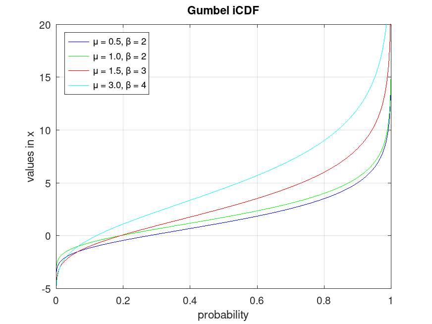
Example: 1
Plot various iCDFs from the Gumbel distribution
 p = 0.001:0.001:0.999;
 x1 = gumbelinv (p, 0.5, 2);
 x2 = gumbelinv (p, 1.0, 2);
 x3 = gumbelinv (p, 1.5, 3);
 x4 = gumbelinv (p, 3.0, 4);
 plot (p, x1, '-b', p, x2, '-g', p, x3, '-r', p, x4, '-c')
 grid on
 ylim ([-5, 20])
 legend ({'μ = 0.5, β = 2', 'μ = 1.0, β = 2', ...
          'μ = 1.5, β = 3', 'μ = 3.0, β = 4'}, 'location', 'northwest')
 title ('Gumbel iCDF')
 xlabel ('probability')
 ylabel ('values in x')