Categories &
Functions List
- BetaDistribution
- BinomialDistribution
- BirnbaumSaundersDistribution
- BurrDistribution
- ExponentialDistribution
- ExtremeValueDistribution
- GammaDistribution
- GeneralizedExtremeValueDistribution
- GeneralizedParetoDistribution
- HalfNormalDistribution
- InverseGaussianDistribution
- LogisticDistribution
- LoglogisticDistribution
- LognormalDistribution
- LoguniformDistribution
- MultinomialDistribution
- NakagamiDistribution
- NegativeBinomialDistribution
- NormalDistribution
- PiecewiseLinearDistribution
- PoissonDistribution
- RayleighDistribution
- RicianDistribution
- tLocationScaleDistribution
- TriangularDistribution
- UniformDistribution
- WeibullDistribution
- betafit
- betalike
- binofit
- binolike
- bisafit
- bisalike
- burrfit
- burrlike
- evfit
- evlike
- expfit
- explike
- gamfit
- gamlike
- geofit
- gevfit_lmom
- gevfit
- gevlike
- gpfit
- gplike
- gumbelfit
- gumbellike
- hnfit
- hnlike
- invgfit
- invglike
- logifit
- logilike
- loglfit
- logllike
- lognfit
- lognlike
- nakafit
- nakalike
- nbinfit
- nbinlike
- normfit
- normlike
- poissfit
- poisslike
- raylfit
- rayllike
- ricefit
- ricelike
- tlsfit
- tlslike
- unidfit
- unifit
- wblfit
- wbllike
- betacdf
- betainv
- betapdf
- betarnd
- binocdf
- binoinv
- binopdf
- binornd
- bisacdf
- bisainv
- bisapdf
- bisarnd
- burrcdf
- burrinv
- burrpdf
- burrrnd
- bvncdf
- bvtcdf
- cauchycdf
- cauchyinv
- cauchypdf
- cauchyrnd
- chi2cdf
- chi2inv
- chi2pdf
- chi2rnd
- copulacdf
- copulapdf
- copularnd
- evcdf
- evinv
- evpdf
- evrnd
- expcdf
- expinv
- exppdf
- exprnd
- fcdf
- finv
- fpdf
- frnd
- gamcdf
- gaminv
- gampdf
- gamrnd
- geocdf
- geoinv
- geopdf
- geornd
- gevcdf
- gevinv
- gevpdf
- gevrnd
- gpcdf
- gpinv
- gppdf
- gprnd
- gumbelcdf
- gumbelinv
- gumbelpdf
- gumbelrnd
- hncdf
- hninv
- hnpdf
- hnrnd
- hygecdf
- hygeinv
- hygepdf
- hygernd
- invgcdf
- invginv
- invgpdf
- invgrnd
- iwishpdf
- iwishrnd
- jsucdf
- jsupdf
- laplacecdf
- laplaceinv
- laplacepdf
- laplacernd
- logicdf
- logiinv
- logipdf
- logirnd
- loglcdf
- loglinv
- loglpdf
- loglrnd
- logncdf
- logninv
- lognpdf
- lognrnd
- mnpdf
- mnrnd
- mvncdf
- mvnpdf
- mvnrnd
- mvtcdf
- mvtpdf
- mvtrnd
- mvtcdfqmc
- nakacdf
- nakainv
- nakapdf
- nakarnd
- nbincdf
- nbininv
- nbinpdf
- nbinrnd
- ncfcdf
- ncfinv
- ncfpdf
- ncfrnd
- nctcdf
- nctinv
- nctpdf
- nctrnd
- ncx2cdf
- ncx2inv
- ncx2pdf
- ncx2rnd
- normcdf
- norminv
- normpdf
- normrnd
- plcdf
- plinv
- plpdf
- plrnd
- poisscdf
- poissinv
- poisspdf
- poissrnd
- raylcdf
- raylinv
- raylpdf
- raylrnd
- ricecdf
- riceinv
- ricepdf
- ricernd
- tcdf
- tinv
- tpdf
- trnd
- tlscdf
- tlsinv
- tlspdf
- tlsrnd
- tricdf
- triinv
- tripdf
- trirnd
- unidcdf
- unidinv
- unidpdf
- unidrnd
- unifcdf
- unifinv
- unifpdf
- unifrnd
- vmcdf
- vminv
- vmpdf
- vmrnd
- wblcdf
- wblinv
- wblpdf
- wblrnd
- wienrnd
- wishpdf
- wishrnd
- adtest
- anova
- anova1
- anova2
- anovan
- bartlett_test
- barttest
- binotest
- chi2gof
- chi2test
- correlation_test
- fishertest
- friedman
- hotelling_t2test
- hotelling_t2test2
- kruskalwallis
- kstest
- kstest2
- levene_test
- manova1
- mcnemar_test
- multcompare
- ranksum
- regression_ftest
- regression_ttest
- runstest
- sampsizepwr
- signrank
- signtest
- tiedrank
- ttest
- ttest2
- vartest
- vartest2
- vartestn
- ztest
- ztest2
Function Reference: multcompare
statistics: C = multcompare (STATS)
statistics: C = multcompare (STATS, "name", value)
statistics: [C, M] = multcompare (...)
statistics: [C, M, H] = multcompare (...)
statistics: [C, M, H, GNAMES] = multcompare (...)
statistics: padj = multcompare (p)
statistics: padj = multcompare (p, "ctype", CTYPE)
Perform posthoc multiple comparison tests or p-value adjustments to control the family-wise error rate (FWER) or false discovery rate (FDR).
C = multcompare (STATS) performs a multiple comparison
using a STATS structure that is obtained as output from any of
the following functions: anova1, anova2, anovan, kruskalwallis, and friedman.
The return value C is a matrix with one row per comparison and six
columns. Columns 1-2 are the indices of the two samples being compared.
Columns 3-5 are a lower bound, estimate, and upper bound for their
difference, where the bounds are for 95% confidence intervals. Column 6-8 are
the multiplicity adjusted p-values for each individual comparison, the test
statistic and the degrees of freedom.
All tests by multcompare are two-tailed.
multcompare can take a number of optional parameters as name-value
pairs.
[…] = multcompare (STATS, "alpha", ALPHA)
- ALPHA sets the significance level of null hypothesis significance tests to ALPHA, and the central coverage of two-sided confidence intervals to 100*(1-ALPHA)%. (Default ALPHA is 0.05).
[…] = multcompare (STATS, "ControlGroup", REF)
- REF is the index of the control group to limit comparisons to. The index must be a positive integer scalar value. For each dimension (d) listed in DIM, multcompare uses STATS.grpnames{d}(idx) as the control group. (Default is empty, i.e. [], for full pairwise comparisons)
[…] = multcompare (STATS, "ctype", CTYPE)
-
CTYPE is the type of comparison test to use. In order of increasing
power, the choices are: "bonferroni", "scheffe", "mvt", "holm" (default),
"hochberg", "fdr", or "lsd". The first five methods control the family-wise
error rate. The "fdr" method controls false discovery rate (by the original
Benjamini-Hochberg step-up procedure). The final method, "lsd" (or "none"),
makes no attempt to control the Type 1 error rate of multiple comparisons.
The coverage of confidence intervals are only corrected for multiple
comparisons in the cases where CTYPE is "bonferroni", "scheffe" or
"mvt", which control the Type 1 error rate for simultaneous inference.
The "mvt" method uses the multivariate t distribution to assess the probability or critical value of the maximum statistic across the tests, thereby accounting for correlations among comparisons in the control of the family-wise error rate with simultaneous inference. In the case of pairwise comparisons, it simulates Tukey’s (or the Games-Howell) test, in the case of comparisons with a single control group, it simulates Dunnett’s test. CTYPE values "tukey-kramer" and "hsd" are recognised but set the value of CTYPE and REF to "mvt" and empty respectively. A CTYPE value "dunnett" is recognised but sets the value of CTYPE to "mvt", and if REF is empty, sets REF to 1. Since the algorithm uses a Monte Carlo method (of 1e+06 random samples), you can expect the results to fluctuate slightly with each call to multcompare and the calculations may be slow to complete for a large number of comparisons. If the parallel package is installed and loaded,
multcomparewill automatically accelerate computations by parallel processing. Note that p-values calculated by the "mvt" are truncated at 1e-06.
[…] = multcompare (STATS, "df", DF)
-
DF is an optional scalar value to set the number of degrees of freedom
in the calculation of p-values for the multiple comparison tests. By default,
this value is extracted from the STATS structure of the ANOVA test, but
setting DF maybe necessary to approximate Satterthwaite correction if
anovanwas performed using weights.
[…] = multcompare (STATS, "dim", DIM)
-
DIM is a vector specifying the dimension or dimensions over which the
estimated marginal means are to be calculated. Used only if STATS comes from
anovan. The value [1 3], for example, computes the estimated marginal mean
for each combination of the first and third predictor values. The default is
to compute over the first dimension (i.e. 1). If the specified dimension is,
or includes, a continuous factor then
multcomparewill return an error.
[…] = multcompare (STATS, "estimate", ESTIMATE)
- ESTIMATE is a string specifying the estimates to be compared when computing multiple comparisons after anova2; this argument is ignored by anovan and anova1. Accepted values for ESTIMATE are either "column" (default) to compare column means, or "row" to compare row means. If the model type in anova2 was "linear" or "nested" then only "column" is accepted for ESTIMATE since the row factor is assumed to be a random effect.
[…] = multcompare (STATS, "display", DISPLAY)
- DISPLAY is either "on" (the default): to display a table and graph of the comparisons (e.g. difference between means), their 100*(1-ALPHA)% intervals and multiplicity adjusted p-values in APA style; or "off": to omit the table and graph. On the graph, markers and error bars colored red have multiplicity adjusted p-values < ALPHA, otherwise the markers and error bars are blue.
[…] = multcompare (STATS, "seed", SEED)
- SEED is a scalar value used to initialize the random number generator so that CTYPE "mvt" produces reproducible results.
[C, M, H, GNAMES] = multcompare (…)
returns additional outputs. M is a matrix where columns 1-2 are the
estimated marginal means and their standard errors, and columns 3-4 are lower
and upper bounds of the confidence intervals for the means; the critical
value of the test statistic is scaled by a factor of 2^(-0.5) before
multiplying by the standard errors of the group means so that the intervals
overlap when the difference in means becomes significant at approximately
the level ALPHA. When ALPHA is 0.05, this corresponds to
confidence intervals with 83.4% central coverage. H is a handle to the
figure containing the graph. GNAMES is a cell array with one row for
each group, containing the names of the groups.
padj = multcompare (p) calculates and returns adjusted
p-values (padj) using the Holm-step down Bonferroni procedure to
control the family-wise error rate.
padj = multcompare (p, "ctype", CTYPE) calculates
and returns adjusted p-values (padj) computed using the method
CTYPE. In order of increasing power, CTYPE for p-value adjustment
can be either "bonferroni", "holm" (default), "hochberg", or "fdr". See
above for further information about the CTYPE methods.
See also: anova1, anova2, anovan, kruskalwallis, friedman, fitlm
Source Code: multcompare
Example: 1
Demonstration using balanced one-way ANOVA from anova1
x = ones (50, 4) .* [-2, 0, 1, 5];
randn ('seed', 1); # for reproducibility
x = x + normrnd (0, 2, 50, 4);
groups = {'A', 'B', 'C', 'D'};
[p, tbl, stats] = anova1 (x, groups, 'off');
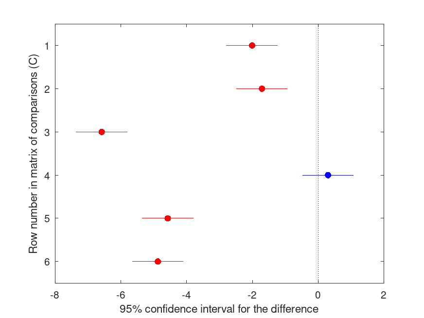
multcompare (stats);
        HOLM Multiple Comparison (Post Hoc) Test for ANOVA1

Group ID  Group ID   LBoundDiff   EstimatedDiff   UBoundDiff   p-value
----------------------------------------------------------------------
    1         2         -2.789        -2.009         -1.228      <.001
    1         3         -2.489        -1.709         -0.928      <.001
    1         4         -7.365        -6.585         -5.804      <.001
    2         3         -0.480         0.300          1.081       .449
    2         4         -5.356        -4.576         -3.795      <.001
    3         4         -5.656        -4.876         -4.095      <.001
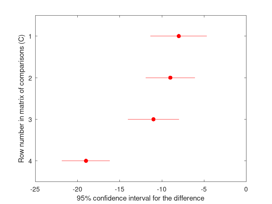
Example: 2
Demonstration using unbalanced one-way ANOVA example from anovan
 dv =  [ 8.706 10.362 11.552  6.941 10.983 10.092  6.421 14.943 15.931 ...
        22.968 18.590 16.567 15.944 21.637 14.492 17.965 18.851 22.891 ...
        22.028 16.884 17.252 18.325 25.435 19.141 21.238 22.196 18.038 ...
        22.628 31.163 26.053 24.419 32.145 28.966 30.207 29.142 33.212 ...
        25.694 ]';
 g = [1 1 1 1 1 1 1 1 2 2 2 2 2 3 3 3 3 3 3 3 3 ...
      4 4 4 4 4 4 4 5 5 5 5 5 5 5 5 5]';
 [P,ATAB, STATS] = anovan (dv, g, 'varnames', 'score', 'display', 'off');
 [C, M, H, GNAMES] = multcompare (STATS, 'dim', 1, 'ctype', 'holm', ...
                                  'ControlGroup', 1, 'display', 'on')
        HOLM Multiple Comparison (Post Hoc) Test for ANOVAN

Group ID  Group ID   LBoundDiff   EstimatedDiff   UBoundDiff   p-value
----------------------------------------------------------------------
    1         2        -11.343        -8.000         -4.657      <.001
    1         3        -11.932        -9.000         -6.068      <.001
    1         4        -14.035       -11.000         -7.965      <.001
    1         5        -21.849       -19.000        -16.151      <.001

C =

   1.0000e+00   2.0000e+00  -1.1343e+01  -8.0000e+00  -4.6572e+00   2.8581e-05  -4.8748e+00   3.2000e+01
   1.0000e+00   3.0000e+00  -1.1932e+01  -9.0000e+00  -6.0682e+00   1.0459e-06  -6.2529e+00   3.2000e+01
   1.0000e+00   4.0000e+00  -1.4035e+01  -1.1000e+01  -7.9654e+00   6.3838e-08  -7.3834e+00   3.2000e+01
   1.0000e+00   5.0000e+00  -2.1849e+01  -1.9000e+01  -1.6151e+01   3.1086e-14  -1.3583e+01   3.2000e+01

M =

   10.0000    1.0178    8.5341   11.4659
   18.0000    1.2874   16.1458   19.8542
   19.0000    1.0178   17.5341   20.4659
   21.0001    1.0880   19.4330   22.5673
   29.0001    0.9595   27.6180   30.3822

H = 1
GNAMES =
  5x1 cell array

    {'score=1'}
    {'score=2'}
    {'score=3'}
    {'score=4'}
    {'score=5'}
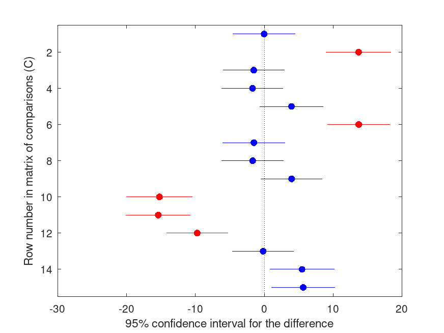
Example: 3
Demonstration using factorial ANCOVA example from anovan
 score = [95.6 82.2 97.2 96.4 81.4 83.6 89.4 83.8 83.3 85.7 ...
 97.2 78.2 78.9 91.8 86.9 84.1 88.6 89.8 87.3 85.4 ...
 81.8 65.8 68.1 70.0 69.9 75.1 72.3 70.9 71.5 72.5 ...
 84.9 96.1 94.6 82.5 90.7 87.0 86.8 93.3 87.6 92.4 ...
 100. 80.5 92.9 84.0 88.4 91.1 85.7 91.3 92.3 87.9 ...
 91.7 88.6 75.8 75.7 75.3 82.4 80.1 86.0 81.8 82.5]';
 treatment = {'yes' 'yes' 'yes' 'yes' 'yes' 'yes' 'yes' 'yes' 'yes' 'yes' ...
              'yes' 'yes' 'yes' 'yes' 'yes' 'yes' 'yes' 'yes' 'yes' 'yes' ...
              'yes' 'yes' 'yes' 'yes' 'yes' 'yes' 'yes' 'yes' 'yes' 'yes' ...
              'no'  'no'  'no'  'no'  'no'  'no'  'no'  'no'  'no'  'no'  ...
              'no'  'no'  'no'  'no'  'no'  'no'  'no'  'no'  'no'  'no'  ...
              'no'  'no'  'no'  'no'  'no'  'no'  'no'  'no'  'no'  'no'}';
 exercise = {'lo'  'lo'  'lo'  'lo'  'lo'  'lo'  'lo'  'lo'  'lo'  'lo'  ...
             'mid' 'mid' 'mid' 'mid' 'mid' 'mid' 'mid' 'mid' 'mid' 'mid' ...
             'hi'  'hi'  'hi'  'hi'  'hi'  'hi'  'hi'  'hi'  'hi'  'hi'  ...
             'lo'  'lo'  'lo'  'lo'  'lo'  'lo'  'lo'  'lo'  'lo'  'lo'  ...
             'mid' 'mid' 'mid' 'mid' 'mid' 'mid' 'mid' 'mid' 'mid' 'mid' ...
             'hi'  'hi'  'hi'  'hi'  'hi'  'hi'  'hi'  'hi'  'hi'  'hi'}';
 age = [59 65 70 66 61 65 57 61 58 55 62 61 60 59 55 57 60 63 62 57 ...
 58 56 57 59 59 60 55 53 55 58 68 62 61 54 59 63 60 67 60 67 ...
 75 54 57 62 65 60 58 61 65 57 56 58 58 58 52 53 60 62 61 61]';
 [P, ATAB, STATS] = anovan (score, {treatment, exercise, age}, 'model', ...
                            [1 0 0; 0 1 0; 0 0 1; 1 1 0], 'continuous', 3, ...
                            'sstype', 'h', 'display', 'off', 'contrasts', ...
                            {'simple','poly',''});
 [C, M, H, GNAMES] = multcompare (STATS, 'dim', [1 2], 'ctype', 'holm', ...
                                  'display', 'on')
        HOLM Multiple Comparison (Post Hoc) Test for ANOVAN

Group ID  Group ID   LBoundDiff   EstimatedDiff   UBoundDiff   p-value
----------------------------------------------------------------------
    1         2         -4.544        -0.017          4.509      1.000
    1         3          8.963        13.703         18.443      <.001
    1         4         -6.002        -1.529          2.945      1.000
    1         5         -6.174        -1.701          2.771      1.000
    1         6         -0.692         3.957          8.605       .662
    2         3          9.166        13.721         18.276      <.001
    2         4         -6.060        -1.511          3.038      1.000
    2         5         -6.195        -1.684          2.828      1.000
    2         6         -0.533         3.974          8.481       .662
    3         4        -20.018       -15.232        -10.446      <.001
    3         5        -20.112       -15.404        -10.697      <.001
    3         6        -14.228        -9.747         -5.265      <.001
    4         5         -4.650        -0.172          4.305      1.000
    4         6          0.798         5.485         10.172       .204
    5         6          1.035         5.658         10.280       .174

C =

   1.0000e+00   2.0000e+00  -4.5437e+00  -1.7457e-02   4.5087e+00   1.0000e+00  -7.7360e-03   5.3000e+01
   1.0000e+00   3.0000e+00   8.9634e+00   1.3703e+01   1.8443e+01   4.5333e-06   5.7988e+00   5.3000e+01
   1.0000e+00   4.0000e+00  -6.0019e+00  -1.5286e+00   2.9447e+00   1.0000e+00  -6.8538e-01   5.3000e+01
   1.0000e+00   5.0000e+00  -6.1735e+00  -1.7011e+00   2.7714e+00   1.0000e+00  -7.6287e-01   5.3000e+01
   1.0000e+00   6.0000e+00  -6.9212e-01   3.9565e+00   8.6051e+00   6.6201e-01   1.7071e+00   5.3000e+01
   2.0000e+00   3.0000e+00   9.1656e+00   1.3721e+01   1.8276e+01   2.0212e-06   6.0416e+00   5.3000e+01
   2.0000e+00   4.0000e+00  -6.0600e+00  -1.5111e+00   3.0378e+00   1.0000e+00  -6.6630e-01   5.3000e+01
   2.0000e+00   5.0000e+00  -6.1953e+00  -1.6836e+00   2.8281e+00   1.0000e+00  -7.4847e-01   5.3000e+01
   2.0000e+00   6.0000e+00  -5.3340e-01   3.9740e+00   8.4813e+00   6.6201e-01   1.7684e+00   5.3000e+01
   3.0000e+00   4.0000e+00  -2.0018e+01  -1.5232e+01  -1.0446e+01   6.1827e-07  -6.3835e+00   5.3000e+01
   3.0000e+00   5.0000e+00  -2.0112e+01  -1.5404e+01  -1.0697e+01   3.4083e-07  -6.5634e+00   5.3000e+01
   3.0000e+00   6.0000e+00  -1.4228e+01  -9.7468e+00  -5.2654e+00   6.5704e-04  -4.3623e+00   5.3000e+01
   4.0000e+00   5.0000e+00  -4.6499e+00  -1.7249e-01   4.3050e+00   1.0000e+00  -7.7268e-02   5.3000e+01
   4.0000e+00   6.0000e+00   7.9808e-01   5.4851e+00   1.0172e+01   2.0411e-01   2.3473e+00   5.3000e+01
   5.0000e+00   6.0000e+00   1.0354e+00   5.6576e+00   1.0280e+01   1.7402e-01   2.4550e+00   5.3000e+01

M =

   86.9788    1.6031   84.7051   89.2525
   86.9962    1.5774   84.7590   89.2334
   73.2755    1.6514   70.9334   75.6176
   88.5074    1.6166   86.2146   90.8002
   88.6799    1.5948   86.4180   90.9417
   83.0223    1.6130   80.7346   85.3100

H = 1
GNAMES =
  6x1 cell array

    {'X1=yes, X2=lo' }
    {'X1=yes, X2=mid'}
    {'X1=yes, X2=hi' }
    {'X1=no, X2=lo'  }
    {'X1=no, X2=mid' }
    {'X1=no, X2=hi'  }
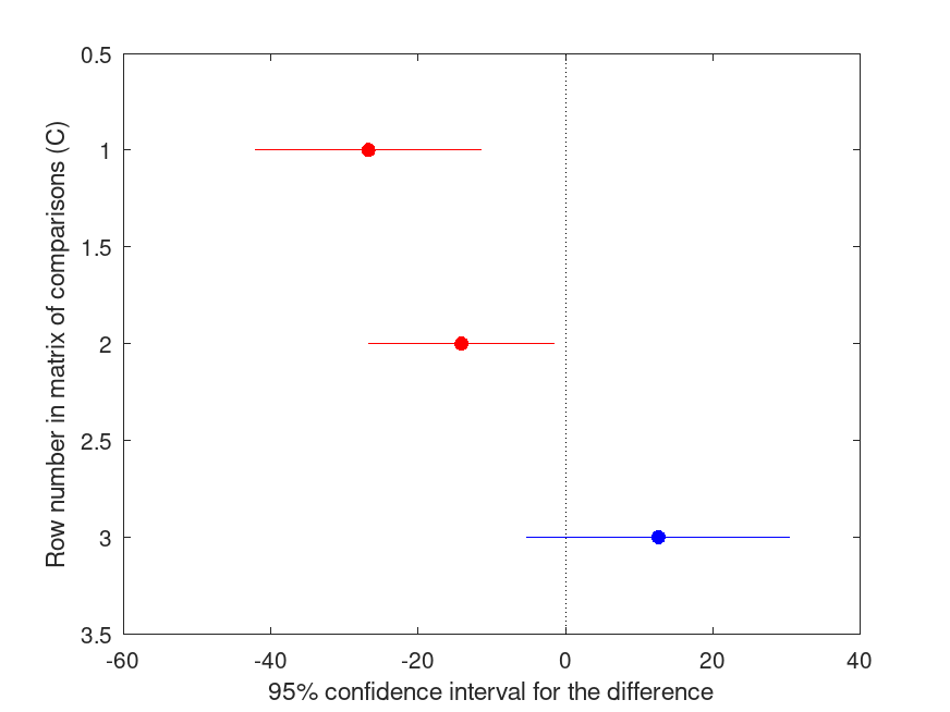
Example: 4
Demonstration using one-way ANOVA from anovan, with fit by weighted least squares to account for heteroskedasticity.
 g = [1, 1, 1, 1, 1, 1, 1, 1, ...
      2, 2, 2, 2, 2, 2, 2, 2, ...
      3, 3, 3, 3, 3, 3, 3, 3]';
 y = [13, 16, 16,  7, 11,  5,  1,  9, ...
      10, 25, 66, 43, 47, 56,  6, 39, ...
      11, 39, 26, 35, 25, 14, 24, 17]';
 [P,ATAB,STATS] = anovan (y, g, 'display', 'off');
 fitted = STATS.X * STATS.coeffs(:,1); # fitted values
 b = polyfit (fitted, abs (STATS.resid), 1);
 v = polyval (b, fitted);  # Variance as a function of the fitted values
 [P,ATAB,STATS] = anovan (y, g, 'weights', v.^-1, 'display', 'off');
 [C, M] =  multcompare (STATS, 'display', 'on', 'ctype', 'mvt')
        MVT Multiple Comparison (Post Hoc) Test for ANOVAN

Group ID  Group ID   LBoundDiff   EstimatedDiff   UBoundDiff   p-value
----------------------------------------------------------------------
    1         2        -42.087       -26.750        -11.413      <.001
    1         3        -26.797       -14.125         -1.453       .027
    2         3         -5.228        12.625         30.478       .199

C =

   1.0000e+00   2.0000e+00  -4.2087e+01  -2.6750e+01  -1.1413e+01   7.2100e-04  -4.3716e+00   2.1000e+01
   1.0000e+00   3.0000e+00  -2.6797e+01  -1.4125e+01  -1.4527e+00   2.7444e-02  -2.7937e+00   2.1000e+01
   2.0000e+00   3.0000e+00  -5.2276e+00   1.2625e+01   3.0478e+01   1.9866e-01   1.7725e+00   2.1000e+01

M =

    9.7500    2.4770    5.3600   14.1400
   36.5000    5.5953   26.5835   46.4165
   23.8750    4.4076   16.0634   31.6866
Example: 5
Demonstration of p-value adjustments to control the false discovery rate Data from Westfall (1997) JASA. 92(437):299-306
 p = [.005708; .023544; .024193; .044895; ...
       .048805; .221227; .395867; .693051; .775755];
 padj = multcompare (p,'ctype','fdr')
padj =

   0.051372
   0.072579
   0.072579
   0.087849
   0.087849
   0.331840
   0.508972
   0.775755
   0.775755