Categories &
Functions List
- BetaDistribution
- BinomialDistribution
- BirnbaumSaundersDistribution
- BurrDistribution
- ExponentialDistribution
- ExtremeValueDistribution
- GammaDistribution
- GeneralizedExtremeValueDistribution
- GeneralizedParetoDistribution
- HalfNormalDistribution
- InverseGaussianDistribution
- LogisticDistribution
- LoglogisticDistribution
- LognormalDistribution
- LoguniformDistribution
- MultinomialDistribution
- NakagamiDistribution
- NegativeBinomialDistribution
- NormalDistribution
- PiecewiseLinearDistribution
- PoissonDistribution
- RayleighDistribution
- RicianDistribution
- tLocationScaleDistribution
- TriangularDistribution
- UniformDistribution
- WeibullDistribution
- betafit
- betalike
- binofit
- binolike
- bisafit
- bisalike
- burrfit
- burrlike
- evfit
- evlike
- expfit
- explike
- gamfit
- gamlike
- geofit
- gevfit_lmom
- gevfit
- gevlike
- gpfit
- gplike
- gumbelfit
- gumbellike
- hnfit
- hnlike
- invgfit
- invglike
- logifit
- logilike
- loglfit
- logllike
- lognfit
- lognlike
- nakafit
- nakalike
- nbinfit
- nbinlike
- normfit
- normlike
- poissfit
- poisslike
- raylfit
- rayllike
- ricefit
- ricelike
- tlsfit
- tlslike
- unidfit
- unifit
- wblfit
- wbllike
- betacdf
- betainv
- betapdf
- betarnd
- binocdf
- binoinv
- binopdf
- binornd
- bisacdf
- bisainv
- bisapdf
- bisarnd
- burrcdf
- burrinv
- burrpdf
- burrrnd
- bvncdf
- bvtcdf
- cauchycdf
- cauchyinv
- cauchypdf
- cauchyrnd
- chi2cdf
- chi2inv
- chi2pdf
- chi2rnd
- copulacdf
- copulapdf
- copularnd
- evcdf
- evinv
- evpdf
- evrnd
- expcdf
- expinv
- exppdf
- exprnd
- fcdf
- finv
- fpdf
- frnd
- gamcdf
- gaminv
- gampdf
- gamrnd
- geocdf
- geoinv
- geopdf
- geornd
- gevcdf
- gevinv
- gevpdf
- gevrnd
- gpcdf
- gpinv
- gppdf
- gprnd
- gumbelcdf
- gumbelinv
- gumbelpdf
- gumbelrnd
- hncdf
- hninv
- hnpdf
- hnrnd
- hygecdf
- hygeinv
- hygepdf
- hygernd
- invgcdf
- invginv
- invgpdf
- invgrnd
- iwishpdf
- iwishrnd
- jsucdf
- jsupdf
- laplacecdf
- laplaceinv
- laplacepdf
- laplacernd
- logicdf
- logiinv
- logipdf
- logirnd
- loglcdf
- loglinv
- loglpdf
- loglrnd
- logncdf
- logninv
- lognpdf
- lognrnd
- mnpdf
- mnrnd
- mvncdf
- mvnpdf
- mvnrnd
- mvtcdf
- mvtpdf
- mvtrnd
- mvtcdfqmc
- nakacdf
- nakainv
- nakapdf
- nakarnd
- nbincdf
- nbininv
- nbinpdf
- nbinrnd
- ncfcdf
- ncfinv
- ncfpdf
- ncfrnd
- nctcdf
- nctinv
- nctpdf
- nctrnd
- ncx2cdf
- ncx2inv
- ncx2pdf
- ncx2rnd
- normcdf
- norminv
- normpdf
- normrnd
- plcdf
- plinv
- plpdf
- plrnd
- poisscdf
- poissinv
- poisspdf
- poissrnd
- raylcdf
- raylinv
- raylpdf
- raylrnd
- ricecdf
- riceinv
- ricepdf
- ricernd
- tcdf
- tinv
- tpdf
- trnd
- tlscdf
- tlsinv
- tlspdf
- tlsrnd
- tricdf
- triinv
- tripdf
- trirnd
- unidcdf
- unidinv
- unidpdf
- unidrnd
- unifcdf
- unifinv
- unifpdf
- unifrnd
- vmcdf
- vminv
- vmpdf
- vmrnd
- wblcdf
- wblinv
- wblpdf
- wblrnd
- wienrnd
- wishpdf
- wishrnd
- adtest
- anova
- anova1
- anova2
- anovan
- bartlett_test
- barttest
- binotest
- chi2gof
- chi2test
- correlation_test
- fishertest
- friedman
- hotelling_t2test
- hotelling_t2test2
- kruskalwallis
- kstest
- kstest2
- levene_test
- manova1
- mcnemar_test
- multcompare
- ranksum
- regression_ftest
- regression_ttest
- runstest
- sampsizepwr
- signrank
- signtest
- tiedrank
- ttest
- ttest2
- vartest
- vartest2
- vartestn
- ztest
- ztest2
Function Reference: poissfit
statistics: lambdahat = poissfit (x)
statistics: [lambdahat, lambdaci] = poissfit (x)
statistics: [lambdahat, lambdaci] = poissfit (x, alpha)
statistics: [lambdahat, lambdaci] = poissfit (x, alpha, freq)
Estimate parameter and confidence intervals for the Poisson distribution.
lambdahat = poissfit (x) returns the maximum likelihood
estimate of the rate parameter, lambda, of the Poisson distribution
given the data in x. x must be a vector of non-negative values.
[lambdahat, lambdaci] = poissfit (x) returns the 95%
confidence intervals for the parameter estimate.
[lambdahat, lambdaci] = poissfit (x, alpha)
also returns the 100 * (1 - alpha) percent confidence intervals
of the estimated parameter. By default, the optional argument alpha is
0.05 corresponding to 95% confidence intervals. Pass in [] for
alpha to use the default values.
[…] = poissfit (x, alpha, freq) accepts a
frequency vector or matrix, freq, of the same size as x.
freq typically contains integer frequencies for the corresponding
elements in x. freq cannot contain negative values.
Further information about the Poisson distribution can be found at https://en.wikipedia.org/wiki/Poisson_distribution
See also: poisscdf, poissinv, poisspdf, poissrnd, poisslike, poisstat
Source Code: poissfit
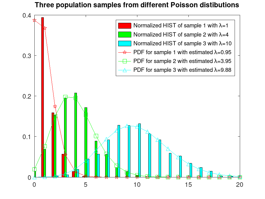
Example: 1
Sample 3 populations from 3 different Poisson distributions
 randp ('seed', 2);    # for reproducibility
 r1 = poissrnd (1, 1000, 1);
 randp ('seed', 2);    # for reproducibility
 r2 = poissrnd (4, 1000, 1);
 randp ('seed', 3);    # for reproducibility
 r3 = poissrnd (10, 1000, 1);
 r = [r1, r2, r3];
Plot them normalized and fix their colors
 hist (r, [0:20], 1);
 h = findobj (gca, 'Type', 'patch');
 set (h(1), 'facecolor', 'c');
 set (h(2), 'facecolor', 'g');
 set (h(3), 'facecolor', 'r');
 hold on
Estimate their lambda parameter
lambdahat = poissfit (r);
Plot their estimated PDFs
 x = [0:20];
 y = poisspdf (x, lambdahat(1));
 plot (x, y, '-pr');
 y = poisspdf (x, lambdahat(2));
 plot (x, y, '-sg');
 y = poisspdf (x, lambdahat(3));
 plot (x, y, '-^c');
 xlim ([0, 20])
 ylim ([0, 0.4])
 legend ({'Normalized HIST of sample 1 with λ=1', ...
          'Normalized HIST of sample 2 with λ=4', ...
          'Normalized HIST of sample 3 with λ=10', ...
          sprintf("PDF for sample 1 with estimated λ=%0.2f", ...
                  lambdahat(1)), ...
          sprintf("PDF for sample 2 with estimated λ=%0.2f", ...
                  lambdahat(2)), ...
          sprintf("PDF for sample 3 with estimated λ=%0.2f", ...
                  lambdahat(3))})
 title ('Three population samples from different Poisson distributions')
 hold off