Categories &
Functions List
- BetaDistribution
- BinomialDistribution
- BirnbaumSaundersDistribution
- BurrDistribution
- ExponentialDistribution
- ExtremeValueDistribution
- GammaDistribution
- GeneralizedExtremeValueDistribution
- GeneralizedParetoDistribution
- HalfNormalDistribution
- InverseGaussianDistribution
- LogisticDistribution
- LoglogisticDistribution
- LognormalDistribution
- LoguniformDistribution
- MultinomialDistribution
- NakagamiDistribution
- NegativeBinomialDistribution
- NormalDistribution
- PiecewiseLinearDistribution
- PoissonDistribution
- RayleighDistribution
- RicianDistribution
- tLocationScaleDistribution
- TriangularDistribution
- UniformDistribution
- WeibullDistribution
- betafit
- betalike
- binofit
- binolike
- bisafit
- bisalike
- burrfit
- burrlike
- evfit
- evlike
- expfit
- explike
- gamfit
- gamlike
- geofit
- gevfit_lmom
- gevfit
- gevlike
- gpfit
- gplike
- gumbelfit
- gumbellike
- hnfit
- hnlike
- invgfit
- invglike
- logifit
- logilike
- loglfit
- logllike
- lognfit
- lognlike
- nakafit
- nakalike
- nbinfit
- nbinlike
- normfit
- normlike
- poissfit
- poisslike
- raylfit
- rayllike
- ricefit
- ricelike
- tlsfit
- tlslike
- unidfit
- unifit
- wblfit
- wbllike
- betacdf
- betainv
- betapdf
- betarnd
- binocdf
- binoinv
- binopdf
- binornd
- bisacdf
- bisainv
- bisapdf
- bisarnd
- burrcdf
- burrinv
- burrpdf
- burrrnd
- bvncdf
- bvtcdf
- cauchycdf
- cauchyinv
- cauchypdf
- cauchyrnd
- chi2cdf
- chi2inv
- chi2pdf
- chi2rnd
- copulacdf
- copulapdf
- copularnd
- evcdf
- evinv
- evpdf
- evrnd
- expcdf
- expinv
- exppdf
- exprnd
- fcdf
- finv
- fpdf
- frnd
- gamcdf
- gaminv
- gampdf
- gamrnd
- geocdf
- geoinv
- geopdf
- geornd
- gevcdf
- gevinv
- gevpdf
- gevrnd
- gpcdf
- gpinv
- gppdf
- gprnd
- gumbelcdf
- gumbelinv
- gumbelpdf
- gumbelrnd
- hncdf
- hninv
- hnpdf
- hnrnd
- hygecdf
- hygeinv
- hygepdf
- hygernd
- invgcdf
- invginv
- invgpdf
- invgrnd
- iwishpdf
- iwishrnd
- jsucdf
- jsupdf
- laplacecdf
- laplaceinv
- laplacepdf
- laplacernd
- logicdf
- logiinv
- logipdf
- logirnd
- loglcdf
- loglinv
- loglpdf
- loglrnd
- logncdf
- logninv
- lognpdf
- lognrnd
- mnpdf
- mnrnd
- mvncdf
- mvnpdf
- mvnrnd
- mvtcdf
- mvtpdf
- mvtrnd
- mvtcdfqmc
- nakacdf
- nakainv
- nakapdf
- nakarnd
- nbincdf
- nbininv
- nbinpdf
- nbinrnd
- ncfcdf
- ncfinv
- ncfpdf
- ncfrnd
- nctcdf
- nctinv
- nctpdf
- nctrnd
- ncx2cdf
- ncx2inv
- ncx2pdf
- ncx2rnd
- normcdf
- norminv
- normpdf
- normrnd
- plcdf
- plinv
- plpdf
- plrnd
- poisscdf
- poissinv
- poisspdf
- poissrnd
- raylcdf
- raylinv
- raylpdf
- raylrnd
- ricecdf
- riceinv
- ricepdf
- ricernd
- tcdf
- tinv
- tpdf
- trnd
- tlscdf
- tlsinv
- tlspdf
- tlsrnd
- tricdf
- triinv
- tripdf
- trirnd
- unidcdf
- unidinv
- unidpdf
- unidrnd
- unifcdf
- unifinv
- unifpdf
- unifrnd
- vmcdf
- vminv
- vmpdf
- vmrnd
- wblcdf
- wblinv
- wblpdf
- wblrnd
- wienrnd
- wishpdf
- wishrnd
- adtest
- anova
- anova1
- anova2
- anovan
- bartlett_test
- barttest
- binotest
- chi2gof
- chi2test
- correlation_test
- fishertest
- friedman
- hotelling_t2test
- hotelling_t2test2
- kruskalwallis
- kstest
- kstest2
- levene_test
- manova1
- mcnemar_test
- multcompare
- ranksum
- regression_ftest
- regression_ttest
- runstest
- sampsizepwr
- signrank
- signtest
- tiedrank
- ttest
- ttest2
- vartest
- vartest2
- vartestn
- ztest
- ztest2
Function Reference: sigma_pts
statistics: pts = sigma_pts (n)
statistics: pts = sigma_pts (n, m)
statistics: pts = sigma_pts (n, m, K)
statistics: pts = sigma_pts (n, m, K, l)
Calculates 2*n+1 sigma points in n dimensions.
Sigma points are used in the unscented transform to estimate the result of applying a given nonlinear transformation to a probability distribution that is characterized only in terms of a finite set of statistics.
If only the dimension n is given the resulting points have zero mean and identity covariance matrix. If the mean m or the covariance matrix K are given, then the resulting points will have those statistics. The factor l scales the points away from the mean. It is useful to tune the accuracy of the unscented transform.
There is no unique way of computing sigma points, this function implements the algorithm described in section 2.6 "The New Filter" pages 40-41 of
Uhlmann, Jeffrey (1995). "Dynamic Map Building and Localization: New Theoretical Foundations". Ph.D. thesis. University of Oxford.
Source Code: sigma_pts
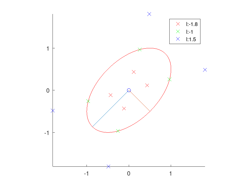
Example: 1
K = [1 0.5; 0.5 1]; # covariance matrix
calculate and build associated ellipse
 [R,S,~] = svd (K);
 theta   = atan2 (R(2,1), R(1,1));
 v       = sqrt (diag (S));
 v       = v .* [cos(theta) sin(theta); -sin(theta) cos(theta)];
 t       = linspace (0, 2*pi, 100).';
 xe      = v(1,1) * cos (t) + v(2,1) * sin (t);
 ye      = v(1,2) * cos (t) + v(2,2) * sin (t);
 figure (1); clf; hold on
Plot ellipse and axes
 line ([0 0; v(:,1).'],[0 0; v(:,2).'])
 plot (xe,ye,'-r');
 col = 'rgb';
 l     = [-1.8 -1 1.5];
 for li = 1:3
  p     = sigma_pts (2, [], K, l(li));
  tmp   = plot (p(2:end,1), p(2:end,2), ['x' col(li)], ...
               p(1,1), p(1,2), ['o' col(li)]);
  h(li) = tmp(1);
 endfor
 hold off
 axis image
 legend (h, arrayfun (@(x) sprintf ("l:%.2g", x), l, 'unif', 0));