Categories &
Functions List
- BetaDistribution
- BinomialDistribution
- BirnbaumSaundersDistribution
- BurrDistribution
- ExponentialDistribution
- ExtremeValueDistribution
- GammaDistribution
- GeneralizedExtremeValueDistribution
- GeneralizedParetoDistribution
- HalfNormalDistribution
- InverseGaussianDistribution
- LogisticDistribution
- LoglogisticDistribution
- LognormalDistribution
- LoguniformDistribution
- MultinomialDistribution
- NakagamiDistribution
- NegativeBinomialDistribution
- NormalDistribution
- PiecewiseLinearDistribution
- PoissonDistribution
- RayleighDistribution
- RicianDistribution
- tLocationScaleDistribution
- TriangularDistribution
- UniformDistribution
- WeibullDistribution
- betafit
- betalike
- binofit
- binolike
- bisafit
- bisalike
- burrfit
- burrlike
- evfit
- evlike
- expfit
- explike
- gamfit
- gamlike
- geofit
- gevfit_lmom
- gevfit
- gevlike
- gpfit
- gplike
- gumbelfit
- gumbellike
- hnfit
- hnlike
- invgfit
- invglike
- logifit
- logilike
- loglfit
- logllike
- lognfit
- lognlike
- nakafit
- nakalike
- nbinfit
- nbinlike
- normfit
- normlike
- poissfit
- poisslike
- raylfit
- rayllike
- ricefit
- ricelike
- tlsfit
- tlslike
- unidfit
- unifit
- wblfit
- wbllike
- betacdf
- betainv
- betapdf
- betarnd
- binocdf
- binoinv
- binopdf
- binornd
- bisacdf
- bisainv
- bisapdf
- bisarnd
- burrcdf
- burrinv
- burrpdf
- burrrnd
- bvncdf
- bvtcdf
- cauchycdf
- cauchyinv
- cauchypdf
- cauchyrnd
- chi2cdf
- chi2inv
- chi2pdf
- chi2rnd
- copulacdf
- copulapdf
- copularnd
- evcdf
- evinv
- evpdf
- evrnd
- expcdf
- expinv
- exppdf
- exprnd
- fcdf
- finv
- fpdf
- frnd
- gamcdf
- gaminv
- gampdf
- gamrnd
- geocdf
- geoinv
- geopdf
- geornd
- gevcdf
- gevinv
- gevpdf
- gevrnd
- gpcdf
- gpinv
- gppdf
- gprnd
- gumbelcdf
- gumbelinv
- gumbelpdf
- gumbelrnd
- hncdf
- hninv
- hnpdf
- hnrnd
- hygecdf
- hygeinv
- hygepdf
- hygernd
- invgcdf
- invginv
- invgpdf
- invgrnd
- iwishpdf
- iwishrnd
- jsucdf
- jsupdf
- laplacecdf
- laplaceinv
- laplacepdf
- laplacernd
- logicdf
- logiinv
- logipdf
- logirnd
- loglcdf
- loglinv
- loglpdf
- loglrnd
- logncdf
- logninv
- lognpdf
- lognrnd
- mnpdf
- mnrnd
- mvncdf
- mvnpdf
- mvnrnd
- mvtcdf
- mvtpdf
- mvtrnd
- mvtcdfqmc
- nakacdf
- nakainv
- nakapdf
- nakarnd
- nbincdf
- nbininv
- nbinpdf
- nbinrnd
- ncfcdf
- ncfinv
- ncfpdf
- ncfrnd
- nctcdf
- nctinv
- nctpdf
- nctrnd
- ncx2cdf
- ncx2inv
- ncx2pdf
- ncx2rnd
- normcdf
- norminv
- normpdf
- normrnd
- plcdf
- plinv
- plpdf
- plrnd
- poisscdf
- poissinv
- poisspdf
- poissrnd
- raylcdf
- raylinv
- raylpdf
- raylrnd
- ricecdf
- riceinv
- ricepdf
- ricernd
- tcdf
- tinv
- tpdf
- trnd
- tlscdf
- tlsinv
- tlspdf
- tlsrnd
- tricdf
- triinv
- tripdf
- trirnd
- unidcdf
- unidinv
- unidpdf
- unidrnd
- unifcdf
- unifinv
- unifpdf
- unifrnd
- vmcdf
- vminv
- vmpdf
- vmrnd
- wblcdf
- wblinv
- wblpdf
- wblrnd
- wienrnd
- wishpdf
- wishrnd
- adtest
- anova
- anova1
- anova2
- anovan
- bartlett_test
- barttest
- binotest
- chi2gof
- chi2test
- correlation_test
- fishertest
- friedman
- hotelling_t2test
- hotelling_t2test2
- kruskalwallis
- kstest
- kstest2
- levene_test
- manova1
- mcnemar_test
- multcompare
- ranksum
- regression_ftest
- regression_ttest
- runstest
- sampsizepwr
- signrank
- signtest
- tiedrank
- ttest
- ttest2
- vartest
- vartest2
- vartestn
- ztest
- ztest2
Function Reference: gevfit
statistics: paramhat = gevfit (x)
statistics: [paramhat, paramci] = gevfit (x)
statistics: [paramhat, paramci] = gevfit (x, alpha)
statistics: [paramhat, paramci] = gevfit (x, alpha, freq)
statistics: [paramhat, paramci] = gevfit (x, alpha, options)
statistics: [paramhat, paramci] = gevfit (x, alpha, freq, options)
Estimate parameters and confidence intervals for the generalized extreme value (GEV) distribution.
paramhat = gevfit (x) returns the maximum likelihood
estimates of the parameters of the GEV distribution given the data in
x. paramhat(1) is the shape parameter, k, and
paramhat(2) is the scale parameter, sigma, and
paramhat(3) is the location parameter, mu.
[paramhat, paramci] = gevfit (x) returns the 95%
confidence intervals for the parameter estimates.
[…] = gevfit (x, alpha) also returns the
100 * (1 - alpha) percent confidence intervals for the
parameter estimates. By default, the optional argument alpha is
0.05 corresponding to 95% confidence intervals. Pass in [] for
alpha to use the default values.
[…] = gevfit (params, x, freq) accepts a
frequency vector, freq, of the same size as x. freq
must contain non-negative integer frequencies for the corresponding elements
in x. By default, or if left empty,
freq = ones (size (x)).
[paramhat, paramci] = gevfit (x, alpha,
 options)
specifies control parameters for the iterative algorithm used
to compute ML estimates with the fminsearch function. options
is a structure with the following fields and their default values:
-
options.Display = "off" -
options.MaxFunEvals = 400 -
options.MaxIter = 200 -
options.TolX = 1e-6
When k < 0, the GEV is the type III extreme value distribution.
When k > 0, the GEV distribution is the type II, or Frechet,
extreme value distribution. If W has a Weibull distribution as
computed by the wblcdf function, then -W has a type III
extreme value distribution and 1/W has a type II extreme value
distribution. In the limit as k approaches 0, the GEV is the
mirror image of the type I extreme value distribution as computed by the
evcdf function.
The mean of the GEV distribution is not finite when k >= 1, and
the variance is not finite when k >= 1/2. The GEV distribution
has positive density only for values of x such that
k * (x - mu) / sigma > -1.
Further information about the generalized extreme value distribution can be found at https://en.wikipedia.org/wiki/Generalized_extreme_value_distribution
See also: gevcdf, gevinv, gevpdf, gevrnd, gevlike, gevstat
Source Code: gevfit
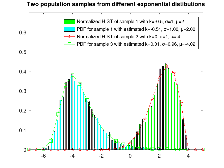
Example: 1
Sample 2 populations from 2 different exponential distributions
 rand ('seed', 1);   # for reproducibility
 r1 = gevrnd (-0.5, 1, 2, 5000, 1);
 rand ('seed', 2);   # for reproducibility
 r2 = gevrnd (0, 1, -4, 5000, 1);
 r = [r1, r2];
Plot them normalized and fix their colors
 hist (r, 50, 5);
 h = findobj (gca, 'Type', 'patch');
 set (h(1), 'facecolor', 'c');
 set (h(2), 'facecolor', 'g');
 hold on
Estimate their k, sigma, and mu parameters
 k_sigma_muA = gevfit (r(:,1));
 k_sigma_muB = gevfit (r(:,2));
Plot their estimated PDFs
 x = [-10:0.5:20];
 y = gevpdf (x, k_sigma_muA(1), k_sigma_muA(2), k_sigma_muA(3));
 plot (x, y, '-pr');
 y = gevpdf (x, k_sigma_muB(1), k_sigma_muB(2), k_sigma_muB(3));
 plot (x, y, '-sg');
 ylim ([0, 0.7])
 xlim ([-7, 5])
 legend ({'Normalized HIST of sample 1 with k=-0.5, σ=1, μ=2', ...
          'Normalized HIST of sample 2 with k=0, σ=1, μ=-4',
     sprintf("PDF for sample 1 with estimated k=%0.2f, σ=%0.2f, μ=%0.2f", ...
                 k_sigma_muA(1), k_sigma_muA(2), k_sigma_muA(3)), ...
     sprintf("PDF for sample 3 with estimated k=%0.2f, σ=%0.2f, μ=%0.2f", ...
                 k_sigma_muB(1), k_sigma_muB(2), k_sigma_muB(3))})
 title ('Two population samples from different exponential distributions')
 hold off