Categories &
Functions List
- BetaDistribution
- BinomialDistribution
- BirnbaumSaundersDistribution
- BurrDistribution
- ExponentialDistribution
- ExtremeValueDistribution
- GammaDistribution
- GeneralizedExtremeValueDistribution
- GeneralizedParetoDistribution
- HalfNormalDistribution
- InverseGaussianDistribution
- LogisticDistribution
- LoglogisticDistribution
- LognormalDistribution
- LoguniformDistribution
- MultinomialDistribution
- NakagamiDistribution
- NegativeBinomialDistribution
- NormalDistribution
- PiecewiseLinearDistribution
- PoissonDistribution
- RayleighDistribution
- RicianDistribution
- tLocationScaleDistribution
- TriangularDistribution
- UniformDistribution
- WeibullDistribution
- betafit
- betalike
- binofit
- binolike
- bisafit
- bisalike
- burrfit
- burrlike
- evfit
- evlike
- expfit
- explike
- gamfit
- gamlike
- geofit
- gevfit_lmom
- gevfit
- gevlike
- gpfit
- gplike
- gumbelfit
- gumbellike
- hnfit
- hnlike
- invgfit
- invglike
- logifit
- logilike
- loglfit
- logllike
- lognfit
- lognlike
- nakafit
- nakalike
- nbinfit
- nbinlike
- normfit
- normlike
- poissfit
- poisslike
- raylfit
- rayllike
- ricefit
- ricelike
- tlsfit
- tlslike
- unidfit
- unifit
- wblfit
- wbllike
- betacdf
- betainv
- betapdf
- betarnd
- binocdf
- binoinv
- binopdf
- binornd
- bisacdf
- bisainv
- bisapdf
- bisarnd
- burrcdf
- burrinv
- burrpdf
- burrrnd
- bvncdf
- bvtcdf
- cauchycdf
- cauchyinv
- cauchypdf
- cauchyrnd
- chi2cdf
- chi2inv
- chi2pdf
- chi2rnd
- copulacdf
- copulapdf
- copularnd
- evcdf
- evinv
- evpdf
- evrnd
- expcdf
- expinv
- exppdf
- exprnd
- fcdf
- finv
- fpdf
- frnd
- gamcdf
- gaminv
- gampdf
- gamrnd
- geocdf
- geoinv
- geopdf
- geornd
- gevcdf
- gevinv
- gevpdf
- gevrnd
- gpcdf
- gpinv
- gppdf
- gprnd
- gumbelcdf
- gumbelinv
- gumbelpdf
- gumbelrnd
- hncdf
- hninv
- hnpdf
- hnrnd
- hygecdf
- hygeinv
- hygepdf
- hygernd
- invgcdf
- invginv
- invgpdf
- invgrnd
- iwishpdf
- iwishrnd
- jsucdf
- jsupdf
- laplacecdf
- laplaceinv
- laplacepdf
- laplacernd
- logicdf
- logiinv
- logipdf
- logirnd
- loglcdf
- loglinv
- loglpdf
- loglrnd
- logncdf
- logninv
- lognpdf
- lognrnd
- mnpdf
- mnrnd
- mvncdf
- mvnpdf
- mvnrnd
- mvtcdf
- mvtpdf
- mvtrnd
- mvtcdfqmc
- nakacdf
- nakainv
- nakapdf
- nakarnd
- nbincdf
- nbininv
- nbinpdf
- nbinrnd
- ncfcdf
- ncfinv
- ncfpdf
- ncfrnd
- nctcdf
- nctinv
- nctpdf
- nctrnd
- ncx2cdf
- ncx2inv
- ncx2pdf
- ncx2rnd
- normcdf
- norminv
- normpdf
- normrnd
- plcdf
- plinv
- plpdf
- plrnd
- poisscdf
- poissinv
- poisspdf
- poissrnd
- raylcdf
- raylinv
- raylpdf
- raylrnd
- ricecdf
- riceinv
- ricepdf
- ricernd
- tcdf
- tinv
- tpdf
- trnd
- tlscdf
- tlsinv
- tlspdf
- tlsrnd
- tricdf
- triinv
- tripdf
- trirnd
- unidcdf
- unidinv
- unidpdf
- unidrnd
- unifcdf
- unifinv
- unifpdf
- unifrnd
- vmcdf
- vminv
- vmpdf
- vmrnd
- wblcdf
- wblinv
- wblpdf
- wblrnd
- wienrnd
- wishpdf
- wishrnd
- adtest
- anova
- anova1
- anova2
- anovan
- bartlett_test
- barttest
- binotest
- chi2gof
- chi2test
- correlation_test
- fishertest
- friedman
- hotelling_t2test
- hotelling_t2test2
- kruskalwallis
- kstest
- kstest2
- levene_test
- manova1
- mcnemar_test
- multcompare
- ranksum
- regression_ftest
- regression_ttest
- runstest
- sampsizepwr
- signrank
- signtest
- tiedrank
- ttest
- ttest2
- vartest
- vartest2
- vartestn
- ztest
- ztest2
Function Reference: hnfit
statistics: [paramhat, paramci] = hnfit (x, mu)
statistics: [paramhat, paramci] = hnfit (x, mu, alpha)
statistics: [paramhat, paramci] = hnfit (x, mu, alpha, freq)
Estimate parameters and confidence intervals for the half-normal distribution.
paramhat = hnfit (x, mu) returns the maximum
likelihood estimates of the parameters of the half-normal distribution given
the data in vector x and the location parameter mu.
paramhat(1) is the location parameter, mu, and
paramhat(2) is the scale parameter, sigma. Although
mu is returned in the estimated paramhat, hnfit does not
estimate the location parameter mu, and it must be assumed to be known,
given as a fixed parameter in input argument mu.
[paramhat, paramci] = hnfit (x, mu) returns
the 95% confidence intervals for the estimated scale parameter sigma.
The first column of paramci includes the location parameter mu
without any confidence bounds.
[…] = hnfit (x, alpha) also returns the
100 * (1 - alpha) percent confidence intervals of the estimated
scale parameter. By default, the optional argument alpha is 0.05
corresponding to 95% confidence intervals.
[…] = hnfit (params, x, freq) accepts a
frequency vector, freq, of the same size as x. freq
must contain non-negative integer frequencies for the corresponding elements
in x. By default, or if left empty,
freq = ones (size (x)).
The half-normal CDF is only defined for x >= mu.
Further information about the half-normal distribution can be found at https://en.wikipedia.org/wiki/Half-normal_distribution
See also: hncdf, hninv, hnpdf, hnrnd, hnlike, hnstat
Source Code: hnfit
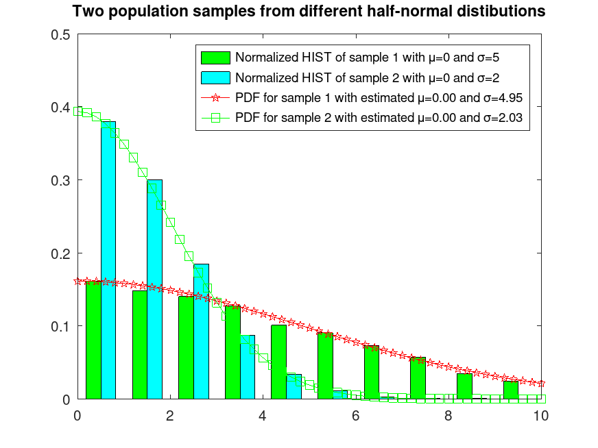
Example: 1
Sample 2 populations from different half-normal distributions
 rand ('seed', 1);   # for reproducibility
 r1 = hnrnd (0, 5, 5000, 1);
 rand ('seed', 2);   # for reproducibility
 r2 = hnrnd (0, 2, 5000, 1);
 r = [r1, r2];
Plot them normalized and fix their colors
 hist (r, [0.5:20], 1);
 h = findobj (gca, 'Type', 'patch');
 set (h(1), 'facecolor', 'c');
 set (h(2), 'facecolor', 'g');
 hold on
Estimate their shape parameters
 mu_sigmaA = hnfit (r(:,1), 0);
 mu_sigmaB = hnfit (r(:,2), 0);
Plot their estimated PDFs
 x = [0:0.2:10];
 y = hnpdf (x, mu_sigmaA(1), mu_sigmaA(2));
 plot (x, y, '-pr');
 y = hnpdf (x, mu_sigmaB(1), mu_sigmaB(2));
 plot (x, y, '-sg');
 xlim ([0, 10])
 ylim ([0, 0.5])
 legend ({'Normalized HIST of sample 1 with μ=0 and σ=5', ...
          'Normalized HIST of sample 2 with μ=0 and σ=2', ...
          sprintf("PDF for sample 1 with estimated μ=%0.2f and σ=%0.2f", ...
                  mu_sigmaA(1), mu_sigmaA(2)), ...
          sprintf("PDF for sample 2 with estimated μ=%0.2f and σ=%0.2f", ...
                  mu_sigmaB(1), mu_sigmaB(2))})
 title ('Two population samples from different half-normal distributions')
 hold off