Categories &
Functions List
- adtest
- anova
- anova1
- anova2
- anovan
- ansaribradley
- barttest
- binotest
- chi2gof
- chi2test
- correlation_test
- detectdrift
- dwtest
- fishertest
- friedman
- hotelling_t2test
- hotelling_t2test2
- jbtest
- knntest
- kruskalwallis
- kstest
- kstest2
- lillietest
- manova1
- mcnemar_test
- meanEffectSize
- mmdtest
- multcompare
- ranksum
- regression_ftest
- regression_ttest
- runstest
- signrank
- signtest
- stats.drift.DriftDiagnostics
- swtest
- ttest
- ttest2
- vartest
- vartest2
- vartestn
- ztest
- ztest2
- CompactLinearModel
- CoxModel
- coxphfit
- fitcox
- fitglm
- fitglme
- fitlm
- fitlme
- fitlmematrix
- fitnlm
- fitrm
- GeneralizedLinearMixedModel
- GeneralizedLinearModel
- glmfit
- glmval
- invpred
- lasso
- lassoglm
- LinearFormula
- LinearMixedModel
- LinearModel
- logistic_regression
- mnrfit
- mnrval
- monotone_smooth
- mvregress
- mvregresslike
- nlinfit
- nlparci
- nlpredci
- NonLinearModel
- plsregress
- regress
- regress_gp
- RepeatedMeasuresModel
- ridge
- robustfit
- stepwisefit
- stepwiseglm
- stepwiselm
- ClassificationBaggedEnsemble
- ClassificationDiscriminant
- ClassificationECOC
- ClassificationEnsemble
- ClassificationGAM
- ClassificationKernel
- ClassificationKNN
- ClassificationLinear
- ClassificationNaiveBayes
- ClassificationNeuralNetwork
- ClassificationPartitionedECOC
- ClassificationPartitionedEnsemble
- ClassificationPartitionedKernel
- ClassificationPartitionedLinear
- ClassificationPartitionedModel
- ClassificationSVM
- ClassificationTree
- CompactClassificationDiscriminant
- CompactClassificationECOC
- CompactClassificationEnsemble
- CompactClassificationGAM
- CompactClassificationNaiveBayes
- CompactClassificationNeuralNetwork
- CompactClassificationSVM
- CompactClassificationTree
- CompactRegressionGAM
- CompactRegressionEnsemble
- CompactRegressionGP
- CompactRegressionNeuralNetwork
- CompactRegressionSVM
- CompactRegressionTree
- CompactTreeBagger
- designecoc
- fcnnpredict
- fcnntrain
- fitcdiscr
- fitcecoc
- fitcensemble
- fitcgam
- fitckernel
- fitcknn
- fitclinear
- fitcnb
- fitcnet
- fitcsvm
- fitctree
- fitrensemble
- fitrgam
- fitrgp
- fitrkernel
- fitrlinear
- fitrnet
- fitrsvm
- fitrtree
- gamboostinter
- gamboostpairs
- gamboostpredict
- gamboosttrain
- gampredict
- gamtrain
- partialDependence
- plotPartialDependence
- PredictiveModel
- RegressionBaggedEnsemble
- RegressionEnsemble
- RegressionGAM
- RegressionGP
- RegressionKernel
- RegressionLinear
- RegressionNeuralNetwork
- RegressionPartitionedEnsemble
- RegressionPartitionedKernel
- RegressionPartitionedLinear
- RegressionPartitionedModel
- RegressionSVM
- RegressionTree
- lime
- shapley
- svmpredict
- svmtrain
- templateDiscriminant
- templateEnsemble
- templateKernel
- templateKNN
- templateLinear
- templateNaiveBayes
- templateSVM
- templateTree
- TreeBagger
- treepredict
- treetrain
- paretotails
- prob.ProbabilityDistribution
- prob.BetaDistribution
- prob.BinomialDistribution
- prob.BirnbaumSaundersDistribution
- prob.BurrDistribution
- prob.ExponentialDistribution
- prob.ExtremeValueDistribution
- prob.GammaDistribution
- prob.GeneralizedExtremeValueDistribution
- prob.GeneralizedParetoDistribution
- prob.HalfNormalDistribution
- prob.InverseGaussianDistribution
- prob.KernelDistribution
- prob.LogisticDistribution
- prob.LoglogisticDistribution
- prob.LognormalDistribution
- prob.LoguniformDistribution
- prob.MultinomialDistribution
- prob.NakagamiDistribution
- prob.NegativeBinomialDistribution
- prob.NormalDistribution
- prob.PiecewiseLinearDistribution
- prob.PoissonDistribution
- prob.RayleighDistribution
- prob.RicianDistribution
- prob.StableDistribution
- prob.tLocationScaleDistribution
- prob.TriangularDistribution
- prob.UniformDistribution
- prob.WeibullDistribution
- betafit
- betalike
- binofit
- binolike
- bisafit
- bisalike
- burrfit
- burrlike
- copulafit
- evfit
- evlike
- expfit
- explike
- gamfit
- gamlike
- geofit
- gevfit
- gevlike
- gevfit_lmom
- gpfit
- gplike
- gumbelfit
- gumbellike
- hnfit
- hnlike
- invgfit
- invglike
- logifit
- logilike
- loglfit
- logllike
- lognfit
- lognlike
- nakafit
- nakalike
- nbinfit
- nbinlike
- normfit
- normlike
- poissfit
- poisslike
- raylfit
- rayllike
- ricefit
- ricelike
- stblfit
- stbllike
- tlsfit
- tlslike
- unidfit
- unifit
- wblfit
- wbllike
- betacdf
- betainv
- betapdf
- betarnd
- binocdf
- binoinv
- binopdf
- binornd
- bisacdf
- bisainv
- bisapdf
- bisarnd
- burrcdf
- burrinv
- burrpdf
- burrrnd
- bvncdf
- bvtcdf
- cauchycdf
- cauchyinv
- cauchypdf
- cauchyrnd
- chi2cdf
- chi2inv
- chi2pdf
- chi2rnd
- copulacdf
- copulapdf
- copularnd
- evcdf
- evinv
- evpdf
- evrnd
- expcdf
- expinv
- exppdf
- exprnd
- fcdf
- finv
- fpdf
- frnd
- gamcdf
- gaminv
- gampdf
- gamrnd
- geocdf
- geoinv
- geopdf
- geornd
- gevcdf
- gevinv
- gevpdf
- gevrnd
- gpcdf
- gpinv
- gppdf
- gprnd
- gumbelcdf
- gumbelinv
- gumbelpdf
- gumbelrnd
- hncdf
- hninv
- hnpdf
- hnrnd
- hygecdf
- hygeinv
- hygepdf
- hygernd
- invgcdf
- invginv
- invgpdf
- invgrnd
- iwishpdf
- iwishrnd
- jsucdf
- jsupdf
- laplacecdf
- laplaceinv
- laplacepdf
- laplacernd
- logicdf
- logiinv
- logipdf
- logirnd
- loglcdf
- loglinv
- loglpdf
- loglrnd
- logncdf
- logninv
- lognpdf
- lognrnd
- mnpdf
- mnrnd
- mvncdf
- mvnpdf
- mvnrnd
- mvtcdf
- mvtpdf
- mvtrnd
- nakacdf
- nakainv
- nakapdf
- nakarnd
- nbincdf
- nbininv
- nbinpdf
- nbinrnd
- ncfcdf
- ncfinv
- ncfpdf
- ncfrnd
- nctcdf
- nctinv
- nctpdf
- nctrnd
- ncx2cdf
- ncx2inv
- ncx2pdf
- ncx2rnd
- normcdf
- norminv
- normpdf
- normrnd
- plcdf
- plinv
- plpdf
- plrnd
- poisscdf
- poissinv
- poisspdf
- poissrnd
- raylcdf
- raylinv
- raylpdf
- raylrnd
- ricecdf
- riceinv
- ricepdf
- ricernd
- stblcdf
- stblinv
- stblpdf
- stblrnd
- stdrcdf
- stdrinv
- stdrpdf
- stdrrnd
- tcdf
- tinv
- tpdf
- trnd
- tlscdf
- tlsinv
- tlspdf
- tlsrnd
- tricdf
- triinv
- tripdf
- trirnd
- unidcdf
- unidinv
- unidpdf
- unidrnd
- unifcdf
- unifinv
- unifpdf
- unifrnd
- vmcdf
- vminv
- vmpdf
- vmrnd
- wblcdf
- wblinv
- wblpdf
- wblrnd
- wienrnd
- wishpdf
- wishrnd
- betastat
- binostat
- bisastat
- burrstat
- chi2stat
- copulaparam
- copulastat
- evstat
- expstat
- fstat
- gamstat
- geostat
- gevstat
- gpstat
- gumbelstat
- hnstat
- hygestat
- invgstat
- logistat
- loglstat
- lognstat
- nakastat
- nbinstat
- ncfstat
- nctstat
- ncx2stat
- normstat
- plstat
- poisstat
- raylstat
- ricestat
- stdrstat
- tlsstat
- tristat
- tstat
- unidstat
- unifstat
- wblstat
- andrewsplot
- bar3
- bar3h
- biplot
- boxchart
- boxplot
- cdfplot
- dendrogram
- ecdfhist
- einstein
- gardnerAltmanPlot
- glyphplot
- gplotmatrix
- gscatter
- heatmap
- hist3
- histfit
- manovacluster
- normplot
- parallelcoords
- parallelplot
- ppplot
- probplot
- qqplot
- scatterhist
- scatterhistogram
- silhouette
- stats.chart.BoxChart
- stats.chart.HeatmapChart
- stats.chart.ParallelCoordinatesPlot
- stats.chart.ScatterHistogramChart
- swarmchart
- violin
- wblplot
Function Reference: jackknife
statistics: jackstat = jackknife (E, x)
statistics: jackstat = jackknife (E, x, …)
statistics: jackstat = jackknife (…, 'Options', options)
Compute jackknife estimates of a parameter taking one or more given samples as parameters.
In particular, E is the estimator to be jackknifed as a function name, handle, or inline function, and x is the sample for which the estimate is to be taken. Each row of x is an observation, and a row vector is taken as a column of them. The i-th row of jackstat holds the estimator’s value on x with its i-th row omitted, reshaped to a row, so an estimator returning m values gives an n×m matrix for n observations, and a scalar estimator a column vector. Every sample must give the estimator’s result the same number of elements as the whole of x does. With fewer than two observations there is nothing to omit, and jackstat is the estimator’s value on x itself.
jackstat (i,:) = E (x([1:i-1, i+1:end],:)) |
Depending on the number of samples to be used, the estimator must have the appropriate form:
-
If only one sample is used, then the estimator need not be concerned with
cell arrays, for example jackknifing the standard deviation of a sample can
be performed with
jackstat = jackknife (@std, rand (100, 1)). -
If several samples are used, an estimator that takes as many inputs, or
declares
varargin, receives each sample as an argument of its own, as in MATLAB. A scalar is passed to every call unchanged, and the other samples must all have the same number of rows, the same row being omitted from each:
jackstat = jackknife (@(x, y) std (x) / var (y), rand (100, 1), randn (100, 1)) |
An estimator declaring exactly one input instead receives the samples as the elements of a cell array, in their order of appearance, and the samples must all have the same number of rows. This form is an Octave extension. An estimator written for it that also declares an optional second input receives the samples as separate arguments.
 jackstat = jackknife (@(x) std(x{1})/var(x{2}),
 rand (100, 1), randn (100, 1))
|
'Options' takes an options structure, as made by statset,
for MATLAB compatibility; it changes nothing, the samples being evaluated
one after another.
If all goes well, a theoretical value P for the parameter is already known, n is the sample size,
t = n * E(x) - (n - 1) *
 mean(jackstat)
and
v = sumsq(n * E(x) - (n - 1) *
 jackstat - t) / (n * (n - 1))
then
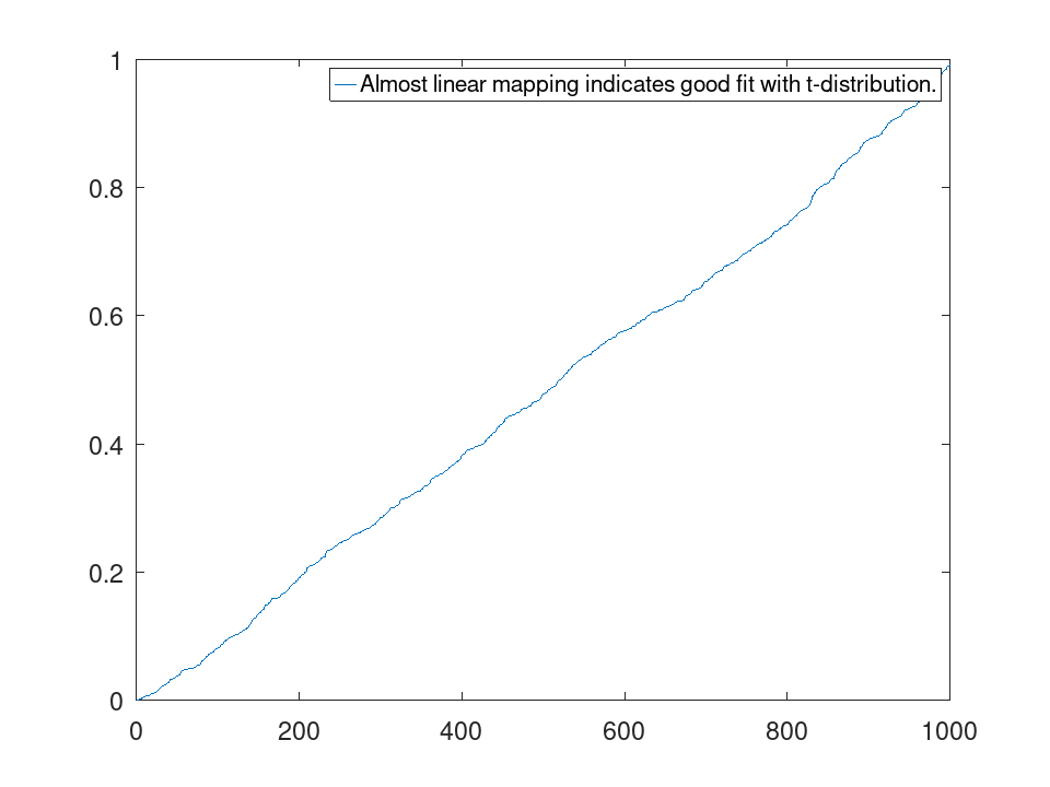
(t-P)/sqrt(v) should follow a t-distribution with
n-1 degrees of freedom.
Jackknifing is a well known method to reduce bias. Further details can be found in:
References
- Rupert G. Miller. The jackknife - a review. Biometrika (1974), 61(1):1-15. doi:10.1093/biomet/61.1.1
- Rupert G. Miller. Jackknifing Variances. Ann. Math. Statist. (1968), Volume 39, Number 2, 567-582. doi:10.1214/aoms/1177698418
Source Code: jackknife
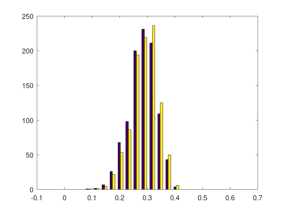
 rng (42);
 for k = 1:1000
   x = rand (10, 1);
   s(k) = std (x);
   jackstat = jackknife (@std, x);
   j(k) = 10 * std (x) - 9 * mean (jackstat);
 endfor
 figure ();
 hist ([s', j'], 0:sqrt (1/12)/10:2*sqrt (1/12))
 rng (42);
 for k = 1:1000
   x = randn (1, 50);
   y = rand (1, 50);
   jackstat = jackknife (@(x) std (x{1})/std (x{2}), y, x);
   j(k) = 50 * std (y) / std (x) - 49 * mean (jackstat);
   v(k) = sumsq ((50 * std (y) / std (x) - 49 * jackstat) - j(k)) / (50 * 49);
 endfor
 t = (j - sqrt (1 / 12)) ./ sqrt (v);
 figure ();
 plot (sort (tcdf (t, 49)), ...
       '-;Almost linear mapping indicates good fit with t-distribution.;')
Jackknife the correlation of two samples, each handed to the estimator as an argument of its own, and correct it for bias
 rng (42);
 x = randn (30, 1);
 y = x + randn (30, 1);
 n = numel (x);
 r = corr (x, y);
 jackstat = jackknife (@(a, b) corr (a, b), x, y);
 bias = (n - 1) * (mean (jackstat) - r)
bias = 5.1710e-03
se = sqrt ((n - 1) / n * sumsq (jackstat - mean (jackstat)))
se = 0.1067
r_corrected = r - bias
r_corrected = 0.6880