Categories &
Functions List
- BetaDistribution
- BinomialDistribution
- BirnbaumSaundersDistribution
- BurrDistribution
- ExponentialDistribution
- ExtremeValueDistribution
- GammaDistribution
- GeneralizedExtremeValueDistribution
- GeneralizedParetoDistribution
- HalfNormalDistribution
- InverseGaussianDistribution
- LogisticDistribution
- LoglogisticDistribution
- LognormalDistribution
- LoguniformDistribution
- MultinomialDistribution
- NakagamiDistribution
- NegativeBinomialDistribution
- NormalDistribution
- PiecewiseLinearDistribution
- PoissonDistribution
- RayleighDistribution
- RicianDistribution
- tLocationScaleDistribution
- TriangularDistribution
- UniformDistribution
- WeibullDistribution
- betafit
- betalike
- binofit
- binolike
- bisafit
- bisalike
- burrfit
- burrlike
- evfit
- evlike
- expfit
- explike
- gamfit
- gamlike
- geofit
- gevfit_lmom
- gevfit
- gevlike
- gpfit
- gplike
- gumbelfit
- gumbellike
- hnfit
- hnlike
- invgfit
- invglike
- logifit
- logilike
- loglfit
- logllike
- lognfit
- lognlike
- nakafit
- nakalike
- nbinfit
- nbinlike
- normfit
- normlike
- poissfit
- poisslike
- raylfit
- rayllike
- ricefit
- ricelike
- tlsfit
- tlslike
- unidfit
- unifit
- wblfit
- wbllike
- betacdf
- betainv
- betapdf
- betarnd
- binocdf
- binoinv
- binopdf
- binornd
- bisacdf
- bisainv
- bisapdf
- bisarnd
- burrcdf
- burrinv
- burrpdf
- burrrnd
- bvncdf
- bvtcdf
- cauchycdf
- cauchyinv
- cauchypdf
- cauchyrnd
- chi2cdf
- chi2inv
- chi2pdf
- chi2rnd
- copulacdf
- copulapdf
- copularnd
- evcdf
- evinv
- evpdf
- evrnd
- expcdf
- expinv
- exppdf
- exprnd
- fcdf
- finv
- fpdf
- frnd
- gamcdf
- gaminv
- gampdf
- gamrnd
- geocdf
- geoinv
- geopdf
- geornd
- gevcdf
- gevinv
- gevpdf
- gevrnd
- gpcdf
- gpinv
- gppdf
- gprnd
- gumbelcdf
- gumbelinv
- gumbelpdf
- gumbelrnd
- hncdf
- hninv
- hnpdf
- hnrnd
- hygecdf
- hygeinv
- hygepdf
- hygernd
- invgcdf
- invginv
- invgpdf
- invgrnd
- iwishpdf
- iwishrnd
- jsucdf
- jsupdf
- laplacecdf
- laplaceinv
- laplacepdf
- laplacernd
- logicdf
- logiinv
- logipdf
- logirnd
- loglcdf
- loglinv
- loglpdf
- loglrnd
- logncdf
- logninv
- lognpdf
- lognrnd
- mnpdf
- mnrnd
- mvncdf
- mvnpdf
- mvnrnd
- mvtcdf
- mvtpdf
- mvtrnd
- mvtcdfqmc
- nakacdf
- nakainv
- nakapdf
- nakarnd
- nbincdf
- nbininv
- nbinpdf
- nbinrnd
- ncfcdf
- ncfinv
- ncfpdf
- ncfrnd
- nctcdf
- nctinv
- nctpdf
- nctrnd
- ncx2cdf
- ncx2inv
- ncx2pdf
- ncx2rnd
- normcdf
- norminv
- normpdf
- normrnd
- plcdf
- plinv
- plpdf
- plrnd
- poisscdf
- poissinv
- poisspdf
- poissrnd
- raylcdf
- raylinv
- raylpdf
- raylrnd
- ricecdf
- riceinv
- ricepdf
- ricernd
- tcdf
- tinv
- tpdf
- trnd
- tlscdf
- tlsinv
- tlspdf
- tlsrnd
- tricdf
- triinv
- tripdf
- trirnd
- unidcdf
- unidinv
- unidpdf
- unidrnd
- unifcdf
- unifinv
- unifpdf
- unifrnd
- vmcdf
- vminv
- vmpdf
- vmrnd
- wblcdf
- wblinv
- wblpdf
- wblrnd
- wienrnd
- wishpdf
- wishrnd
- adtest
- anova
- anova1
- anova2
- anovan
- bartlett_test
- barttest
- binotest
- chi2gof
- chi2test
- correlation_test
- fishertest
- friedman
- hotelling_t2test
- hotelling_t2test2
- kruskalwallis
- kstest
- kstest2
- levene_test
- manova1
- mcnemar_test
- multcompare
- ranksum
- regression_ftest
- regression_ttest
- runstest
- sampsizepwr
- signrank
- signtest
- tiedrank
- ttest
- ttest2
- vartest
- vartest2
- vartestn
- ztest
- ztest2
Function Reference: glmfit
statistics: b = glmfit (X, y, distribution)
statistics: b = glmfit (X, y, distribution, Name, Value)
statistics: [b, dev] = glmfit (…)
statistics: [b, dev, stats] = glmfit (…)
Perform generalized linear model fitting.
b = glmfit (X, y, distribution) returns a
vector b of coefficient estimates for a generalized linear regression
model of the responses in y on the predictors in X, using the
distribution defined in distribution.
- X is an numeric matrix of predictor variables with observations and predictors.
- y is an numeric vector of responses for all supported distributions, except for the ’binomial’ distribution in which case y can be either a numeric or logical vector or an matrix, where the first column contains the number of successes and the second column contains the number of trials.
- distribution is a character vector specifying the distribution of
the response variable. Supported distributions are
'normal','binomial','poisson','gamma', and'inverse gaussian'.
b = glmfit (…, Name, Value) specifies
additional options using Name-Value pair arguments.
| Name | Value | |
|---|---|---|
'B0' | A numeric vector specifying initial values for the coefficient estimates. By default, the initial values are fitted values fitted from the data. | |
'Constant' | A character vector specifying whether to include a constant term in the model. Valid options are "on" (default) and "off". | |
'EstDisp' | A character vector specifying whether to
compute dispersion parameter. Valid options are "on" and "off".
For 'binomial' and 'poisson' distributions the default is
"off", whereas for the 'normal', 'gamma', and
'inverse gaussian' distributions the default is "on". | |
'link' | A character vector specifying the name of a
canonical link function or a numeric scalar for specifying a 'power'
link function. Supported canonical link functions include 'identity'
(default for 'normal' distribution), 'log' (default for
'poisson' distribution), 'logit' (default for
'binomial' distribution), 'probit', 'loglog',
'comploglog', and 'reciprocal' (default for the
'gamma' distribution). The 'power' link function is the
default for the 'inverse gaussian' distribution with .
For custom link functions, the user can provide cell array with three
function handles: the link function, its derivative, and its inverse, or
alternatively a structure S with three fields: S.Link,
S.Derivative, and S.Inverse. Each field can either contain a
function handle or a character vector with the name of an existing function.
All custom link functions must accept a vector of inputs and return a vector
of the same size. | |
'Offset' | A numeric vector of the same length as the response y specifying an offset variable in the fit. It is used as an additional predictor with a coefficient value fixed at 1. | |
'Options' | A scalar structure containing the fields
MaxIter and TolX. MaxIter must be a scalar positive
integer specifying the maximum number of iteration allowed for fitting the
model, and TolX must be a positive scalar value specifying the
termination tolerance. | |
'Weights' | An numeric vector of nonnegative
values, where is the number of observations in X. By default,
it is ones (n, 1). |
[b, dev] = glmfit (…) also returns the deviance of
the fit as a numeric value in dev. Deviance is a generalization of the
residual sum of squares. It measures the goodness of fit compared to a
saturated model.
[b, dev, stats] = glmfit (…) also returns the
structure stats, which contains the model statistics in the following
fields:
-
beta- Coefficient estimates b -
dfe- Degrees of freedom for error -
sfit- Estimated dispersion parameter -
s- Theoretical or estimated dispersion parameter -
estdisp-falsewhen'EstDisp'is'off'andtruewhen'EstDisp'is'on' -
covb- Estimated covariance matrix for b -
se- Vector of standard errors of the coefficient estimates b -
coeffcorr- Correlation matrix for b -
t- statistics for b -
p- -values for b -
resid- Vector of residuals -
residp- Vector of Pearson residuals -
residd- Vector of deviance residuals -
resida- Vector of Anscombe residuals
See also: glmval
Source Code: glmfit
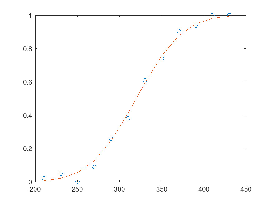
Example: 1
 x = [210, 230, 250, 270, 290, 310, 330, 350, 370, 390, 410, 430]';
 n = [48, 42, 31, 34, 31, 21, 23, 23, 21, 16, 17, 21]';
 y = [1, 2, 0, 3, 8, 8, 14, 17, 19, 15, 17, 21]';
 b = glmfit (x, [y n], 'binomial', 'Link', 'probit');
 yfit = glmval (b, x, 'probit', 'Size', n);
 plot (x, y./n, 'o', x, yfit ./ n, '-')
Example: 2
 load fisheriris
 X = meas (51:end, :);
 y = strcmp ('versicolor', species(51:end));
 b = glmfit (X, y, 'binomial', 'link', 'logit')
b =

   42.6378
    2.4652
    6.6809
   -9.4294
  -18.2861