Categories &
Functions List
- adtest
- anova
- anova1
- anova2
- anovan
- ansaribradley
- barttest
- binotest
- chi2gof
- chi2test
- correlation_test
- detectdrift
- dwtest
- fishertest
- friedman
- hotelling_t2test
- hotelling_t2test2
- jbtest
- knntest
- kruskalwallis
- kstest
- kstest2
- lillietest
- manova1
- mcnemar_test
- meanEffectSize
- mmdtest
- multcompare
- ranksum
- regression_ftest
- regression_ttest
- runstest
- signrank
- signtest
- stats.drift.DriftDiagnostics
- swtest
- ttest
- ttest2
- vartest
- vartest2
- vartestn
- ztest
- ztest2
- CompactLinearModel
- CoxModel
- coxphfit
- fitcox
- fitglm
- fitglme
- fitlm
- fitlme
- fitlmematrix
- fitnlm
- fitrm
- GeneralizedLinearMixedModel
- GeneralizedLinearModel
- glmfit
- glmval
- invpred
- lasso
- lassoglm
- LinearFormula
- LinearMixedModel
- LinearModel
- logistic_regression
- mnrfit
- mnrval
- monotone_smooth
- mvregress
- mvregresslike
- nlinfit
- nlparci
- nlpredci
- NonLinearModel
- plsregress
- regress
- regress_gp
- RepeatedMeasuresModel
- ridge
- robustfit
- stepwisefit
- stepwiseglm
- stepwiselm
- ClassificationBaggedEnsemble
- ClassificationDiscriminant
- ClassificationECOC
- ClassificationEnsemble
- ClassificationGAM
- ClassificationKernel
- ClassificationKNN
- ClassificationLinear
- ClassificationNaiveBayes
- ClassificationNeuralNetwork
- ClassificationPartitionedECOC
- ClassificationPartitionedEnsemble
- ClassificationPartitionedKernel
- ClassificationPartitionedLinear
- ClassificationPartitionedModel
- ClassificationSVM
- ClassificationTree
- CompactClassificationDiscriminant
- CompactClassificationECOC
- CompactClassificationEnsemble
- CompactClassificationGAM
- CompactClassificationNaiveBayes
- CompactClassificationNeuralNetwork
- CompactClassificationSVM
- CompactClassificationTree
- CompactRegressionGAM
- CompactRegressionEnsemble
- CompactRegressionGP
- CompactRegressionNeuralNetwork
- CompactRegressionSVM
- CompactRegressionTree
- CompactTreeBagger
- designecoc
- fcnnpredict
- fcnntrain
- fitcdiscr
- fitcecoc
- fitcensemble
- fitcgam
- fitckernel
- fitcknn
- fitclinear
- fitcnb
- fitcnet
- fitcsvm
- fitctree
- fitrensemble
- fitrgam
- fitrgp
- fitrkernel
- fitrlinear
- fitrnet
- fitrsvm
- fitrtree
- gamboostinter
- gamboostpairs
- gamboostpredict
- gamboosttrain
- gampredict
- gamtrain
- partialDependence
- plotPartialDependence
- PredictiveModel
- RegressionBaggedEnsemble
- RegressionEnsemble
- RegressionGAM
- RegressionGP
- RegressionKernel
- RegressionLinear
- RegressionNeuralNetwork
- RegressionPartitionedEnsemble
- RegressionPartitionedKernel
- RegressionPartitionedLinear
- RegressionPartitionedModel
- RegressionSVM
- RegressionTree
- lime
- shapley
- svmpredict
- svmtrain
- templateDiscriminant
- templateEnsemble
- templateKernel
- templateKNN
- templateLinear
- templateNaiveBayes
- templateSVM
- templateTree
- TreeBagger
- treepredict
- treetrain
- paretotails
- prob.ProbabilityDistribution
- prob.BetaDistribution
- prob.BinomialDistribution
- prob.BirnbaumSaundersDistribution
- prob.BurrDistribution
- prob.ExponentialDistribution
- prob.ExtremeValueDistribution
- prob.GammaDistribution
- prob.GeneralizedExtremeValueDistribution
- prob.GeneralizedParetoDistribution
- prob.HalfNormalDistribution
- prob.InverseGaussianDistribution
- prob.KernelDistribution
- prob.LogisticDistribution
- prob.LoglogisticDistribution
- prob.LognormalDistribution
- prob.LoguniformDistribution
- prob.MultinomialDistribution
- prob.NakagamiDistribution
- prob.NegativeBinomialDistribution
- prob.NormalDistribution
- prob.PiecewiseLinearDistribution
- prob.PoissonDistribution
- prob.RayleighDistribution
- prob.RicianDistribution
- prob.StableDistribution
- prob.tLocationScaleDistribution
- prob.TriangularDistribution
- prob.UniformDistribution
- prob.WeibullDistribution
- betafit
- betalike
- binofit
- binolike
- bisafit
- bisalike
- burrfit
- burrlike
- copulafit
- evfit
- evlike
- expfit
- explike
- gamfit
- gamlike
- geofit
- gevfit
- gevlike
- gevfit_lmom
- gpfit
- gplike
- gumbelfit
- gumbellike
- hnfit
- hnlike
- invgfit
- invglike
- logifit
- logilike
- loglfit
- logllike
- lognfit
- lognlike
- nakafit
- nakalike
- nbinfit
- nbinlike
- normfit
- normlike
- poissfit
- poisslike
- raylfit
- rayllike
- ricefit
- ricelike
- stblfit
- stbllike
- tlsfit
- tlslike
- unidfit
- unifit
- wblfit
- wbllike
- betacdf
- betainv
- betapdf
- betarnd
- binocdf
- binoinv
- binopdf
- binornd
- bisacdf
- bisainv
- bisapdf
- bisarnd
- burrcdf
- burrinv
- burrpdf
- burrrnd
- bvncdf
- bvtcdf
- cauchycdf
- cauchyinv
- cauchypdf
- cauchyrnd
- chi2cdf
- chi2inv
- chi2pdf
- chi2rnd
- copulacdf
- copulapdf
- copularnd
- evcdf
- evinv
- evpdf
- evrnd
- expcdf
- expinv
- exppdf
- exprnd
- fcdf
- finv
- fpdf
- frnd
- gamcdf
- gaminv
- gampdf
- gamrnd
- geocdf
- geoinv
- geopdf
- geornd
- gevcdf
- gevinv
- gevpdf
- gevrnd
- gpcdf
- gpinv
- gppdf
- gprnd
- gumbelcdf
- gumbelinv
- gumbelpdf
- gumbelrnd
- hncdf
- hninv
- hnpdf
- hnrnd
- hygecdf
- hygeinv
- hygepdf
- hygernd
- invgcdf
- invginv
- invgpdf
- invgrnd
- iwishpdf
- iwishrnd
- jsucdf
- jsupdf
- laplacecdf
- laplaceinv
- laplacepdf
- laplacernd
- logicdf
- logiinv
- logipdf
- logirnd
- loglcdf
- loglinv
- loglpdf
- loglrnd
- logncdf
- logninv
- lognpdf
- lognrnd
- mnpdf
- mnrnd
- mvncdf
- mvnpdf
- mvnrnd
- mvtcdf
- mvtpdf
- mvtrnd
- nakacdf
- nakainv
- nakapdf
- nakarnd
- nbincdf
- nbininv
- nbinpdf
- nbinrnd
- ncfcdf
- ncfinv
- ncfpdf
- ncfrnd
- nctcdf
- nctinv
- nctpdf
- nctrnd
- ncx2cdf
- ncx2inv
- ncx2pdf
- ncx2rnd
- normcdf
- norminv
- normpdf
- normrnd
- plcdf
- plinv
- plpdf
- plrnd
- poisscdf
- poissinv
- poisspdf
- poissrnd
- raylcdf
- raylinv
- raylpdf
- raylrnd
- ricecdf
- riceinv
- ricepdf
- ricernd
- stblcdf
- stblinv
- stblpdf
- stblrnd
- stdrcdf
- stdrinv
- stdrpdf
- stdrrnd
- tcdf
- tinv
- tpdf
- trnd
- tlscdf
- tlsinv
- tlspdf
- tlsrnd
- tricdf
- triinv
- tripdf
- trirnd
- unidcdf
- unidinv
- unidpdf
- unidrnd
- unifcdf
- unifinv
- unifpdf
- unifrnd
- vmcdf
- vminv
- vmpdf
- vmrnd
- wblcdf
- wblinv
- wblpdf
- wblrnd
- wienrnd
- wishpdf
- wishrnd
- betastat
- binostat
- bisastat
- burrstat
- chi2stat
- copulaparam
- copulastat
- evstat
- expstat
- fstat
- gamstat
- geostat
- gevstat
- gpstat
- gumbelstat
- hnstat
- hygestat
- invgstat
- logistat
- loglstat
- lognstat
- nakastat
- nbinstat
- ncfstat
- nctstat
- ncx2stat
- normstat
- plstat
- poisstat
- raylstat
- ricestat
- stdrstat
- tlsstat
- tristat
- tstat
- unidstat
- unifstat
- wblstat
- andrewsplot
- bar3
- bar3h
- biplot
- boxchart
- boxplot
- cdfplot
- dendrogram
- ecdfhist
- einstein
- gardnerAltmanPlot
- glyphplot
- gplotmatrix
- gscatter
- heatmap
- hist3
- histfit
- manovacluster
- normplot
- parallelcoords
- parallelplot
- ppplot
- probplot
- qqplot
- scatterhist
- scatterhistogram
- silhouette
- stats.chart.BoxChart
- stats.chart.HeatmapChart
- stats.chart.ParallelCoordinatesPlot
- stats.chart.ScatterHistogramChart
- swarmchart
- violin
- wblplot
Class Definition: LinearModel
statistics: LinearModel
Linear regression model
The LinearModel class represents a least-squares (or, optionally,
robust) linear regression fit of a response variable to one or more
predictor variables. A LinearModel object is returned by the
fitlm function and holds everything about the fit in one place:
the fitted coefficients, the data and specification used to produce
them, and the diagnostics needed to assess the quality of the fit.
The properties of a LinearModel object fall into four groups:
| Group | Properties |
|---|---|
| Coefficient estimates | Coefficients (a table of
estimates, standard errors, t-statistics, and p-values for each term),
CoefficientCovariance, CoefficientNames, and the
coefficient counts NumCoefficients and
NumEstimatedCoefficients. |
| Summary statistics of the fit | DFE,
Fitted, Residuals (raw, Pearson, Studentized, and
standardized), Diagnostics (leverage, Cook’s distance, and other
per-observation influence measures), MSE, RMSE,
Rsquared (ordinary and adjusted), SSE, SSR,
SST, LogLikelihood, ModelCriterion (AIC, BIC, etc.),
and ModelFitVsNullModel (the F-test of the fitted model against an
intercept-only model). |
| Fitting method information | Robust, which records
the weighting function and tuning constant used when the model is fit by
robust regression, and is empty for an ordinary least squares fit, and
Steps, which records the stepwise fitting information whenever
the model was fit using stepwise regression, and is currently always
empty. |
| Input data properties | Formula,
NumObservations, NumPredictors, NumVariables,
ObservationInfo (which observations were used, excluded, missing,
or weighted), ObservationNames, PredictorNames,
ResponseName, VariableInfo, VariableNames, and
Variables. |
A categorical predictor expands to indicator columns, one per level bar
the reference level, which the intercept carries. When the model has no
intercept, the first categorical predictor is given an indicator
for every one of its levels instead, so that its coefficients are the
group means; any further categorical predictor stays reference coded,
which keeps the design full rank. This differs from MATLAB, which omits
the reference level whether or not an intercept is present and so cannot
fit the reference group at all – for a three-level grouping variable
g, MATLAB fits y ~ g - 1 with two coefficients, predicts
exactly 0 for every observation in the omitted group, and reports a
negative R^2. This implementation returns three coefficients, one
per group.
A LinearModel object supports categorical predictors, which are
automatically encoded internally as indicator (dummy) variables,
observation weights for a weighted least squares fit, excluding specific
observations from the fit, and robust regression using iteratively
reweighted least squares. Once fitted, the following methods are
available on a LinearModel object:
| Method | Description |
|---|---|
predict | Predict responses at new predictor values given in a matrix or table, or reproduce the training fitted values when called with no new data. Can also return pointwise or simultaneous confidence or prediction intervals alongside the point predictions. |
feval | Predict responses given predictors as
separate scalar or vector arguments (one per predictor variable) instead
of a single matrix, so a LinearModel object can be evaluated the
same way as a plain function handle. Returns point predictions only. |
random | Simulate new response values at new
predictor locations by adding independent Gaussian noise, drawn from the
estimated error variance MSE, to the fitted response. |
coefCI | Return Wald confidence intervals for every fitted coefficient at a chosen significance level (default 0.05). |
coefTest | Test a linear hypothesis on the fitted coefficients. With no arguments, tests the overall model F-test that all non-intercept coefficients are zero; a custom hypothesis can be given as a contrast matrix and, if needed, right-hand-side values. Returns the p-value, and optionally the F-statistic and its numerator degrees of freedom. |
dwtest | Durbin-Watson test for first-order autocorrelation among the model residuals, with a choice of exact or approximate p-value computation and a one- or two-sided alternative. |
addTerms | Return a new, refitted LinearModel
with terms added to the current model specification, given as a
Wilkinson formula fragment or a terms matrix. Weights, excluded rows,
and categorical encodings carry over automatically; the original model
object is left unmodified. |
removeTerms | Return a new, refitted
LinearModel with terms removed from the current model
specification, given as a Wilkinson formula fragment or a terms matrix.
Weights, excluded rows, and categorical encodings carry over
automatically; the original model object is left unmodified. |
plotResiduals | Plot the model residuals. Default
is a probability density histogram; other supported plot types are
'fitted', 'caseorder', 'lagged',
'probability', and 'observed'. |
plotDiagnostics | Plot per-observation influence
diagnostics. Default is leverage by observation row number; other
supported plot types are 'cookd', 'covratio',
'dfbetas', 'dffits', 's2_i', and
'contour' (standardized residuals against leverage with Cook’s
distance contours). |
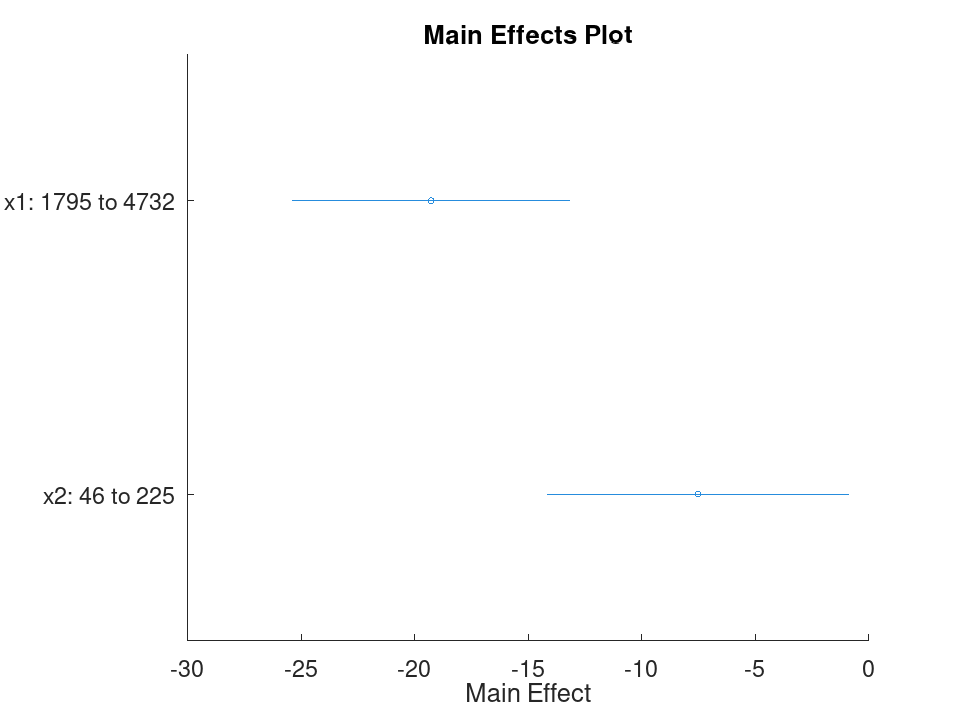
plotEffects | Plot the estimated main effect and 95% confidence interval of each predictor, evaluated between its observed minimum and maximum with all other predictors held at their observed means. |
plotAdjustedResponse | Plot the fitted response against a single predictor, with the other predictors averaged out by averaging the fitted values over the observations used in the fit. |
plotAdded | Plot the incremental effect of one or more terms on the response, after removing the effects of all other terms, along with the fitted line and its 95% confidence bounds. |
plot | Plot a default view of the model. Creates an added variable plot for the whole model when more than one predictor is included, a scatter plot of the data with a fitted curve and 95% confidence bounds when exactly one predictor is included, or a histogram of the residuals when no predictors are included. |
plotInteraction | Plot the main and conditional effects of two predictors, or the adjusted response as a function of one predictor for several fixed values of the other, to visualize whether the two predictors interact. |
compact | Return a CompactLinearModel that
discards the training data and per-observation diagnostics while
retaining the coefficient estimates and fit statistics needed for
prediction and inference. |
anova | Analysis of variance for the fitted model, reporting either the per-term breakdown of sums of squares or a summary table of the model against the total and residual variation. |
step | Improve the fitted model by one or more
steps of stepwise term selection, returning a new, refitted
LinearModel without modifying the original. |
Create a LinearModel object by using the fitlm function or
the class constructor directly.
See also: fitlm
Source Code: LinearModel
The LinearModel class contains the following properties:
A p-by-p numeric matrix of covariance values for the
coefficient estimates, where p is the number of coefficients in
the fitted model as given by NumCoefficients. This property is
read-only.
Simple linear regression with a single predictor. Ten runners record their weekly training distance and their finish time in a 10k race. We fit a straight line through this data and look at the fitted coefficients, then use predict to estimate the finish time for a runner who trains a distance not in the sample.
 Distance = [10; 15; 20; 25; 30; 35; 40; 45; 50; 55];
 Time     = [58; 55; 52; 50; 47; 45; 43; 41; 40; 38];
 X = Distance;
 y = Time;
Fit the model and inspect the estimated slope and intercept.
mdl = fitlm (X, y)
mdl =

  Linear regression model:
      y ~ 1 + x1

  Estimated Coefficients:

  2x4 table

                   Estimate       SE         tStat        pValue
                   ________    _________    ________    ___________

    (Intercept)        61.2     0.654588      93.494    1.91213e-13
    x1                -0.44    0.0184226    -23.8836    1.00609e-08


Number of observations: 10, Error degrees of freedom: 8
Root Mean Squared Error: 0.83666
R-squared: 0.986169,  Adjusted R-Squared: 0.984441
F-statistic vs. constant model: 570.429, p-value = 1.00609e-08
Predict the finish time for a runner training 32 km per week.
ypred = predict (mdl, 32)
ypred = 47.120
Multiple linear regression with two predictors, followed by a confidence interval on the coefficients. Thirteen coffee shops report their weekly foot traffic and the number of items on their menu, along with weekly revenue. We fit a model with both predictors, then use coefCI to see how precisely each coefficient is estimated.
 Traffic = [120; 150; 90; 200; 175; 60; 220; 140; 100; 190; 80; 210; 130];
 MenuSize = [8; 12; 6; 15; 10; 5; 18; 9; 7; 14; 6; 16; 11];
 Revenue = [1450; 1820; 1010; 2400; 2050; 700; 2650; 1700; 1150; ...
            2300; 900; 2500; 1600];
 X = [Traffic, MenuSize];
 y = Revenue;
Fit the model with both predictors together.
mdl = fitlm (X, y)
mdl =

  Linear regression model:
      y ~ 1 + x1 + x2

  Estimated Coefficients:

  3x4 table

                   Estimate       SE        tStat        pValue
                   ________    ________    ________    ___________

    (Intercept)    -47.0932     27.3456    -1.72215       0.115771
    x1              11.4079    0.616078      18.517    4.55169e-09
    x2              11.4344     7.68384     1.48811       0.167562


Number of observations: 13, Error degrees of freedom: 10
Root Mean Squared Error: 32.4551
R-squared: 0.997901,  Adjusted R-Squared: 0.997482
F-statistic vs. constant model: 2377.53, p-value = 4.07061e-14
Check how tight the 95% confidence interval is on each coefficient.
ci = coefCI (mdl)
ci =

  -108.0231    13.8366
    10.0352    12.7806
    -5.6862    28.5551
Growing a model with addTerms and predicting with the richer model. We model fuel economy from the carsmall data set using weight and horsepower as main effects only. addTerms then brings in the weight-horsepower interaction without needing to refit by hand, and predict shows how the estimate for a new car changes once that interaction is included.
 load carsmall
 X = [Weight, Horsepower];
 y = MPG;
Fit the additive model first.
mdl = fitlm (X, y);
Add the interaction between weight and horsepower.
mdl2 = addTerms (mdl, 'x1:x2');
Compare predictions from both models for the same new car.
 Xnew = [3200, 120];
 ypred1 = predict (mdl, Xnew)
ypred1 = 21.719
ypred2 = predict (mdl2, Xnew)
ypred2 = 20.416
Simplifying a model with removeTerms and comparing fit quality. We fit the full Hald cement model with all four ingredients, then use removeTerms to drop the weakest predictor and refit automatically. Comparing SSE before and after shows how little explanatory power that ingredient was actually contributing.
 load hald
 X = ingredients;
 y = heat;
Fit the model with all four ingredients.
mdl = fitlm (X, y);
Drop the third ingredient and refit on the same data.
mdl2 = removeTerms (mdl, 'x3');
Compare how much the error sum of squares changed.
sse_full = mdl.SSE
sse_full = 47.864
sse_reduced = mdl2.SSE
sse_reduced = 47.973
Testing a linear hypothesis and checking residual autocorrelation. Twelve patients are given a drug at different doses over different treatment durations, and a recovery score is recorded. coefTest checks whether the dose and duration coefficients are actually equal, and dwtest separately checks whether the residuals still carry a leftover pattern the model failed to capture.
 Dose     = [10; 15; 20; 25; 30; 35; 12; 18; 22; 28; 32; 38];
 Duration = [5; 7; 9; 11; 13; 15; 6; 8; 10; 12; 14; 16];
 Recovery = [42; 48; 55; 60; 68; 74; 45; 52; 58; 65; 71; 78];
 X = [Dose, Duration];
 y = Recovery;
 mdl = fitlm (X, y);
Test H0: the Dose and Duration coefficients are equal.
 H = [0 1 -1];
 [p, F, r] = coefTest (mdl, H)
p = 0.3535
F = 0.9571
r = 1
Check for autocorrelation left over in the residuals.
[pdw, dw] = dwtest (mdl)
pdw = 0.3658
dw = 2.4432
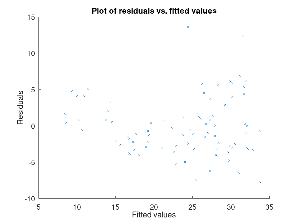
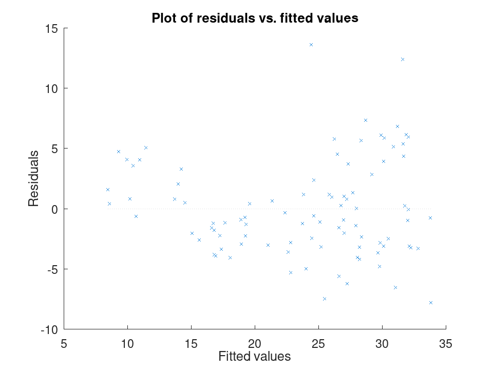
Checking residuals against fitted values. We fit a mileage model on the carsmall data set using weight and horsepower, then plot the raw residuals against the fitted values. A pattern in this plot, rather than a random scatter, would suggest the linear model is missing some curvature in the relationship.
 load carsmall
 X = [Weight, Horsepower];
 y = MPG;
 mdl = fitlm (X, y);
 plotResiduals (mdl, 'fitted')
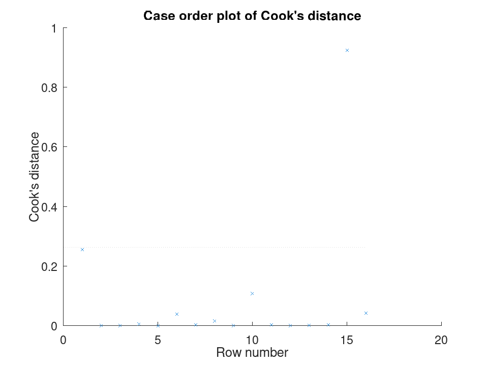
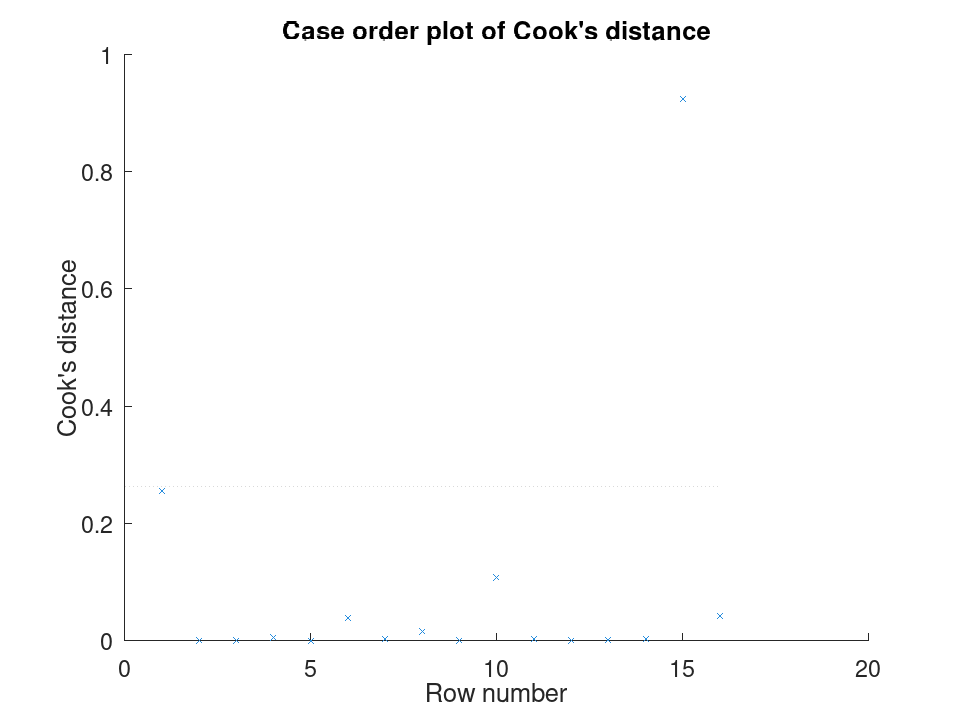
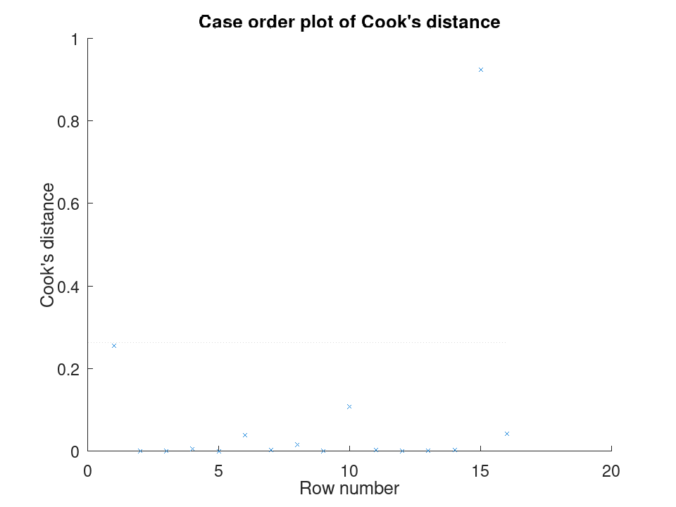
Spotting influential observations with Cook's distance. Sixteen houses are matched by size and age to a sale price, but one house was sold far above what its size and age would predict. After fitting the model, plotDiagnostics with the cookd option highlights that single observation as having outsized influence on the fit.
 Size  = [80; 95; 110; 120; 65; 140; 100; 130; 90; 150; 75; 105; ...
          115; 85; 135; 125];
 Age   = [5; 10; 3; 8; 20; 2; 15; 6; 12; 1; 18; 9; 4; 14; 7; 11];
 Price = [200; 230; 260; 280; 150; 320; 240; 300; 210; 340; 170; ...
          250; 270; 190; 500; 290];
 X = [Size, Age];
 y = Price;
 mdl = fitlm (X, y);
 plotDiagnostics (mdl, 'cookd')
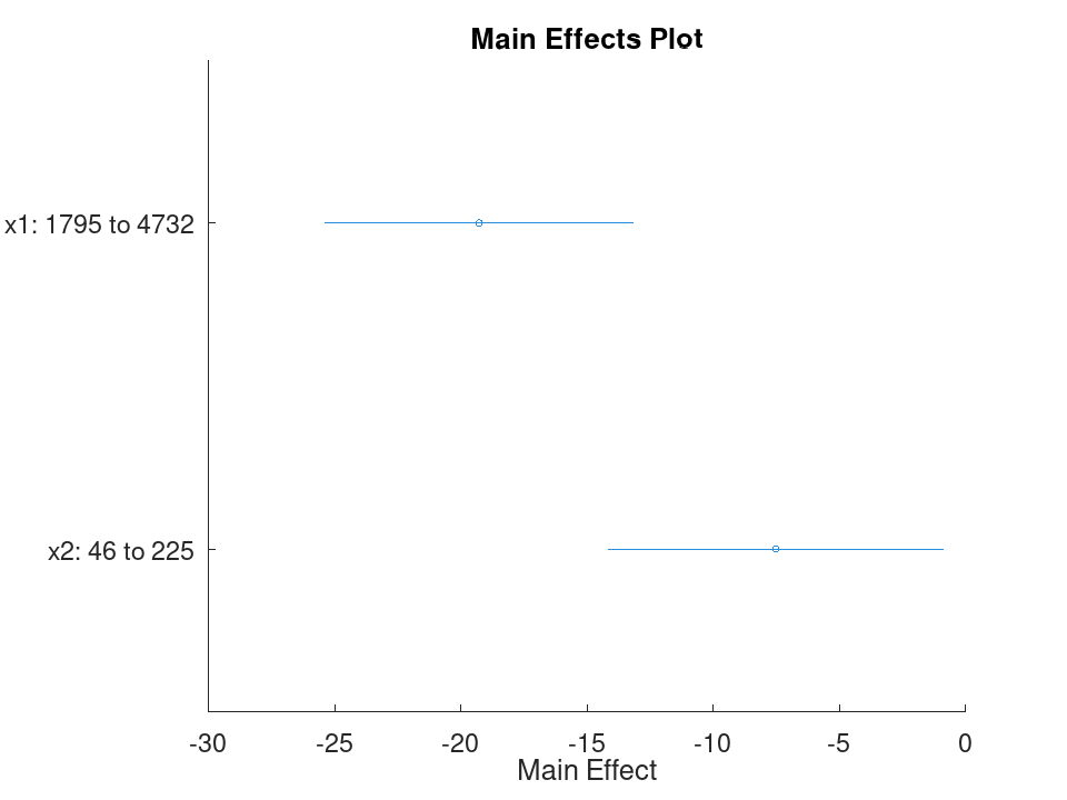
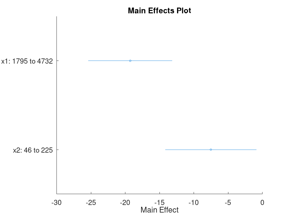
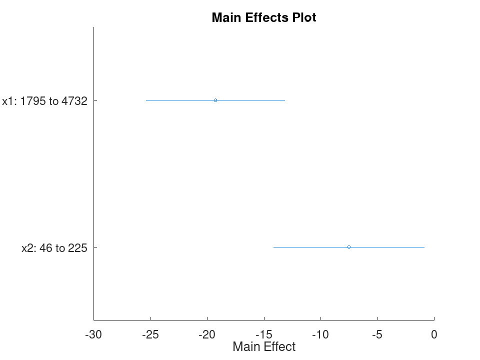
Comparing the size of each predictor's effect, alongside a hypothesis test on the model as a whole. We fit a mileage model on the carsmall data set using weight and horsepower. plotEffects draws each coefficient's estimate with its confidence interval side by side, and coefTest checks whether weight's effect is significantly different from horsepower's.
 load carsmall
 X = [Weight, Horsepower];
 y = MPG;
 mdl = fitlm (X, y);
Visualize the relative size of each predictor's effect.
plotEffects (mdl)
Test whether the two coefficients differ significantly.
 H = [0 1 -1];
 [p, F, r] = coefTest (mdl, H)
p = 0.073643
F = 3.2759
r = 1
A cell array of character vectors, each containing the name of the
corresponding model term (e.g., '(Intercept)', 'x1',
'x1:x2'). This property is read-only.
Simple linear regression with a single predictor. Ten runners record their weekly training distance and their finish time in a 10k race. We fit a straight line through this data and look at the fitted coefficients, then use predict to estimate the finish time for a runner who trains a distance not in the sample.
 Distance = [10; 15; 20; 25; 30; 35; 40; 45; 50; 55];
 Time     = [58; 55; 52; 50; 47; 45; 43; 41; 40; 38];
 X = Distance;
 y = Time;
Fit the model and inspect the estimated slope and intercept.
mdl = fitlm (X, y)
mdl =

  Linear regression model:
      y ~ 1 + x1

  Estimated Coefficients:

  2x4 table

                   Estimate       SE         tStat        pValue
                   ________    _________    ________    ___________

    (Intercept)        61.2     0.654588      93.494    1.91213e-13
    x1                -0.44    0.0184226    -23.8836    1.00609e-08


Number of observations: 10, Error degrees of freedom: 8
Root Mean Squared Error: 0.83666
R-squared: 0.986169,  Adjusted R-Squared: 0.984441
F-statistic vs. constant model: 570.429, p-value = 1.00609e-08
Predict the finish time for a runner training 32 km per week.
ypred = predict (mdl, 32)
ypred = 47.120
Multiple linear regression with two predictors, followed by a confidence interval on the coefficients. Thirteen coffee shops report their weekly foot traffic and the number of items on their menu, along with weekly revenue. We fit a model with both predictors, then use coefCI to see how precisely each coefficient is estimated.
 Traffic = [120; 150; 90; 200; 175; 60; 220; 140; 100; 190; 80; 210; 130];
 MenuSize = [8; 12; 6; 15; 10; 5; 18; 9; 7; 14; 6; 16; 11];
 Revenue = [1450; 1820; 1010; 2400; 2050; 700; 2650; 1700; 1150; ...
            2300; 900; 2500; 1600];
 X = [Traffic, MenuSize];
 y = Revenue;
Fit the model with both predictors together.
mdl = fitlm (X, y)
mdl =

  Linear regression model:
      y ~ 1 + x1 + x2

  Estimated Coefficients:

  3x4 table

                   Estimate       SE        tStat        pValue
                   ________    ________    ________    ___________

    (Intercept)    -47.0932     27.3456    -1.72215       0.115771
    x1              11.4079    0.616078      18.517    4.55169e-09
    x2              11.4344     7.68384     1.48811       0.167562


Number of observations: 13, Error degrees of freedom: 10
Root Mean Squared Error: 32.4551
R-squared: 0.997901,  Adjusted R-Squared: 0.997482
F-statistic vs. constant model: 2377.53, p-value = 4.07061e-14
Check how tight the 95% confidence interval is on each coefficient.
ci = coefCI (mdl)
ci =

  -108.0231    13.8366
    10.0352    12.7806
    -5.6862    28.5551
Growing a model with addTerms and predicting with the richer model. We model fuel economy from the carsmall data set using weight and horsepower as main effects only. addTerms then brings in the weight-horsepower interaction without needing to refit by hand, and predict shows how the estimate for a new car changes once that interaction is included.
 load carsmall
 X = [Weight, Horsepower];
 y = MPG;
Fit the additive model first.
mdl = fitlm (X, y);
Add the interaction between weight and horsepower.
mdl2 = addTerms (mdl, 'x1:x2');
Compare predictions from both models for the same new car.
 Xnew = [3200, 120];
 ypred1 = predict (mdl, Xnew)
ypred1 = 21.719
ypred2 = predict (mdl2, Xnew)
ypred2 = 20.416
Simplifying a model with removeTerms and comparing fit quality. We fit the full Hald cement model with all four ingredients, then use removeTerms to drop the weakest predictor and refit automatically. Comparing SSE before and after shows how little explanatory power that ingredient was actually contributing.
 load hald
 X = ingredients;
 y = heat;
Fit the model with all four ingredients.
mdl = fitlm (X, y);
Drop the third ingredient and refit on the same data.
mdl2 = removeTerms (mdl, 'x3');
Compare how much the error sum of squares changed.
sse_full = mdl.SSE
sse_full = 47.864
sse_reduced = mdl2.SSE
sse_reduced = 47.973
Testing a linear hypothesis and checking residual autocorrelation. Twelve patients are given a drug at different doses over different treatment durations, and a recovery score is recorded. coefTest checks whether the dose and duration coefficients are actually equal, and dwtest separately checks whether the residuals still carry a leftover pattern the model failed to capture.
 Dose     = [10; 15; 20; 25; 30; 35; 12; 18; 22; 28; 32; 38];
 Duration = [5; 7; 9; 11; 13; 15; 6; 8; 10; 12; 14; 16];
 Recovery = [42; 48; 55; 60; 68; 74; 45; 52; 58; 65; 71; 78];
 X = [Dose, Duration];
 y = Recovery;
 mdl = fitlm (X, y);
Test H0: the Dose and Duration coefficients are equal.
 H = [0 1 -1];
 [p, F, r] = coefTest (mdl, H)
p = 0.3535
F = 0.9571
r = 1
Check for autocorrelation left over in the residuals.
[pdw, dw] = dwtest (mdl)
pdw = 0.3658
dw = 2.4432
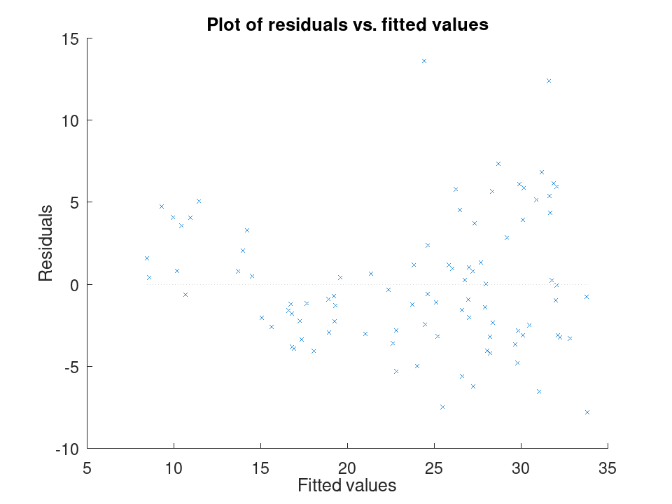
Checking residuals against fitted values. We fit a mileage model on the carsmall data set using weight and horsepower, then plot the raw residuals against the fitted values. A pattern in this plot, rather than a random scatter, would suggest the linear model is missing some curvature in the relationship.
 load carsmall
 X = [Weight, Horsepower];
 y = MPG;
 mdl = fitlm (X, y);
 plotResiduals (mdl, 'fitted')
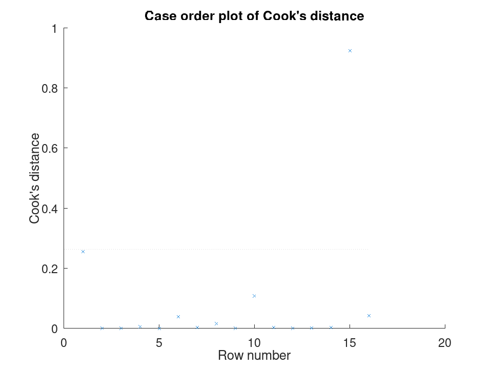
Spotting influential observations with Cook's distance. Sixteen houses are matched by size and age to a sale price, but one house was sold far above what its size and age would predict. After fitting the model, plotDiagnostics with the cookd option highlights that single observation as having outsized influence on the fit.
 Size  = [80; 95; 110; 120; 65; 140; 100; 130; 90; 150; 75; 105; ...
          115; 85; 135; 125];
 Age   = [5; 10; 3; 8; 20; 2; 15; 6; 12; 1; 18; 9; 4; 14; 7; 11];
 Price = [200; 230; 260; 280; 150; 320; 240; 300; 210; 340; 170; ...
          250; 270; 190; 500; 290];
 X = [Size, Age];
 y = Price;
 mdl = fitlm (X, y);
 plotDiagnostics (mdl, 'cookd')
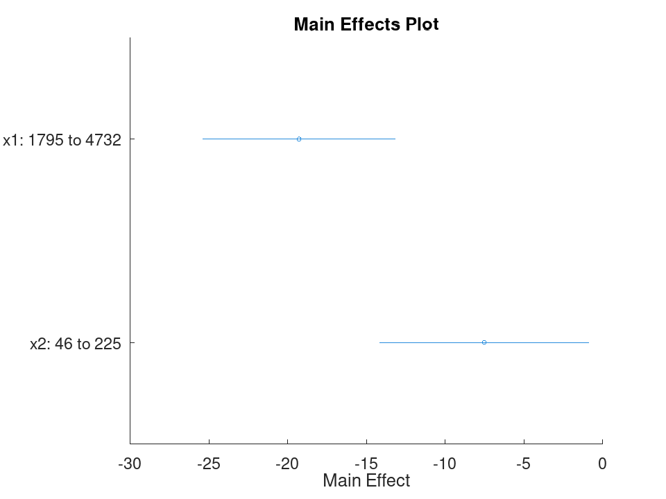
Comparing the size of each predictor's effect, alongside a hypothesis test on the model as a whole. We fit a mileage model on the carsmall data set using weight and horsepower. plotEffects draws each coefficient's estimate with its confidence interval side by side, and coefTest checks whether weight's effect is significantly different from horsepower's.
 load carsmall
 X = [Weight, Horsepower];
 y = MPG;
 mdl = fitlm (X, y);
Visualize the relative size of each predictor's effect.
plotEffects (mdl)
Test whether the two coefficients differ significantly.
 H = [0 1 -1];
 [p, F, r] = coefTest (mdl, H)
p = 0.073643
F = 3.2759
r = 1
A table with one row for each coefficient and four columns:
-
Estimate- estimated coefficient value -
SE- standard error of the estimate -
tStat- t-statistic for a two-sided test -
pValue- p-value for the t-statistic
Coefficients that are dropped due to rank deficiency have
Estimate = 0, SE = 0, tStat = NaN,
pValue = NaN. This property is read-only.
Simple linear regression with a single predictor. Ten runners record their weekly training distance and their finish time in a 10k race. We fit a straight line through this data and look at the fitted coefficients, then use predict to estimate the finish time for a runner who trains a distance not in the sample.
 Distance = [10; 15; 20; 25; 30; 35; 40; 45; 50; 55];
 Time     = [58; 55; 52; 50; 47; 45; 43; 41; 40; 38];
 X = Distance;
 y = Time;
Fit the model and inspect the estimated slope and intercept.
mdl = fitlm (X, y)
mdl =

  Linear regression model:
      y ~ 1 + x1

  Estimated Coefficients:

  2x4 table

                   Estimate       SE         tStat        pValue
                   ________    _________    ________    ___________

    (Intercept)        61.2     0.654588      93.494    1.91213e-13
    x1                -0.44    0.0184226    -23.8836    1.00609e-08


Number of observations: 10, Error degrees of freedom: 8
Root Mean Squared Error: 0.83666
R-squared: 0.986169,  Adjusted R-Squared: 0.984441
F-statistic vs. constant model: 570.429, p-value = 1.00609e-08
Predict the finish time for a runner training 32 km per week.
ypred = predict (mdl, 32)
ypred = 47.120
Multiple linear regression with two predictors, followed by a confidence interval on the coefficients. Thirteen coffee shops report their weekly foot traffic and the number of items on their menu, along with weekly revenue. We fit a model with both predictors, then use coefCI to see how precisely each coefficient is estimated.
 Traffic = [120; 150; 90; 200; 175; 60; 220; 140; 100; 190; 80; 210; 130];
 MenuSize = [8; 12; 6; 15; 10; 5; 18; 9; 7; 14; 6; 16; 11];
 Revenue = [1450; 1820; 1010; 2400; 2050; 700; 2650; 1700; 1150; ...
            2300; 900; 2500; 1600];
 X = [Traffic, MenuSize];
 y = Revenue;
Fit the model with both predictors together.
mdl = fitlm (X, y)
mdl =

  Linear regression model:
      y ~ 1 + x1 + x2

  Estimated Coefficients:

  3x4 table

                   Estimate       SE        tStat        pValue
                   ________    ________    ________    ___________

    (Intercept)    -47.0932     27.3456    -1.72215       0.115771
    x1              11.4079    0.616078      18.517    4.55169e-09
    x2              11.4344     7.68384     1.48811       0.167562


Number of observations: 13, Error degrees of freedom: 10
Root Mean Squared Error: 32.4551
R-squared: 0.997901,  Adjusted R-Squared: 0.997482
F-statistic vs. constant model: 2377.53, p-value = 4.07061e-14
Check how tight the 95% confidence interval is on each coefficient.
ci = coefCI (mdl)
ci =

  -108.0231    13.8366
    10.0352    12.7806
    -5.6862    28.5551
Growing a model with addTerms and predicting with the richer model. We model fuel economy from the carsmall data set using weight and horsepower as main effects only. addTerms then brings in the weight-horsepower interaction without needing to refit by hand, and predict shows how the estimate for a new car changes once that interaction is included.
 load carsmall
 X = [Weight, Horsepower];
 y = MPG;
Fit the additive model first.
mdl = fitlm (X, y);
Add the interaction between weight and horsepower.
mdl2 = addTerms (mdl, 'x1:x2');
Compare predictions from both models for the same new car.
 Xnew = [3200, 120];
 ypred1 = predict (mdl, Xnew)
ypred1 = 21.719
ypred2 = predict (mdl2, Xnew)
ypred2 = 20.416
Simplifying a model with removeTerms and comparing fit quality. We fit the full Hald cement model with all four ingredients, then use removeTerms to drop the weakest predictor and refit automatically. Comparing SSE before and after shows how little explanatory power that ingredient was actually contributing.
 load hald
 X = ingredients;
 y = heat;
Fit the model with all four ingredients.
mdl = fitlm (X, y);
Drop the third ingredient and refit on the same data.
mdl2 = removeTerms (mdl, 'x3');
Compare how much the error sum of squares changed.
sse_full = mdl.SSE
sse_full = 47.864
sse_reduced = mdl2.SSE
sse_reduced = 47.973
Testing a linear hypothesis and checking residual autocorrelation. Twelve patients are given a drug at different doses over different treatment durations, and a recovery score is recorded. coefTest checks whether the dose and duration coefficients are actually equal, and dwtest separately checks whether the residuals still carry a leftover pattern the model failed to capture.
 Dose     = [10; 15; 20; 25; 30; 35; 12; 18; 22; 28; 32; 38];
 Duration = [5; 7; 9; 11; 13; 15; 6; 8; 10; 12; 14; 16];
 Recovery = [42; 48; 55; 60; 68; 74; 45; 52; 58; 65; 71; 78];
 X = [Dose, Duration];
 y = Recovery;
 mdl = fitlm (X, y);
Test H0: the Dose and Duration coefficients are equal.
 H = [0 1 -1];
 [p, F, r] = coefTest (mdl, H)
p = 0.3535
F = 0.9571
r = 1
Check for autocorrelation left over in the residuals.
[pdw, dw] = dwtest (mdl)
pdw = 0.3658
dw = 2.4432
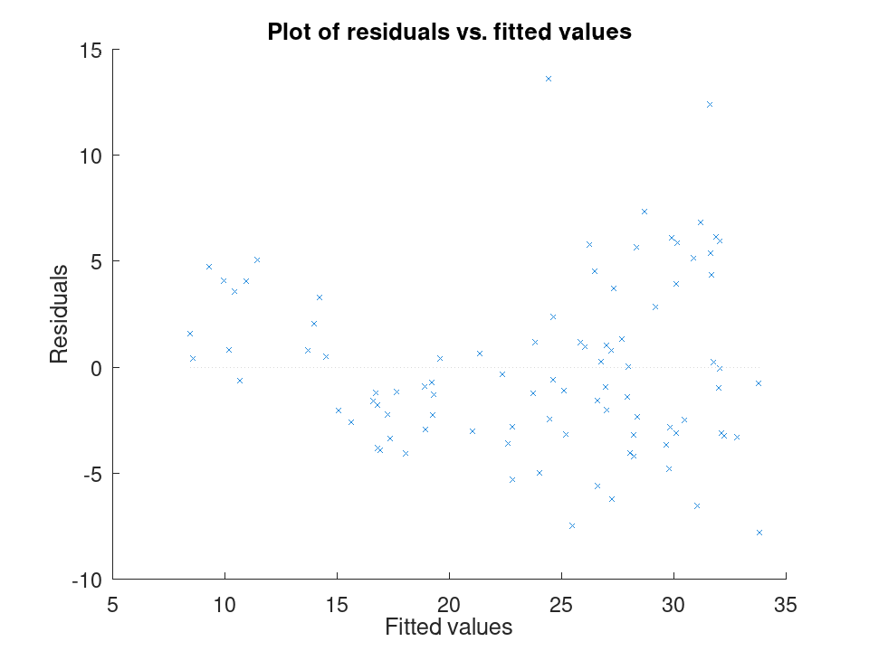
Checking residuals against fitted values. We fit a mileage model on the carsmall data set using weight and horsepower, then plot the raw residuals against the fitted values. A pattern in this plot, rather than a random scatter, would suggest the linear model is missing some curvature in the relationship.
 load carsmall
 X = [Weight, Horsepower];
 y = MPG;
 mdl = fitlm (X, y);
 plotResiduals (mdl, 'fitted')
Spotting influential observations with Cook's distance. Sixteen houses are matched by size and age to a sale price, but one house was sold far above what its size and age would predict. After fitting the model, plotDiagnostics with the cookd option highlights that single observation as having outsized influence on the fit.
 Size  = [80; 95; 110; 120; 65; 140; 100; 130; 90; 150; 75; 105; ...
          115; 85; 135; 125];
 Age   = [5; 10; 3; 8; 20; 2; 15; 6; 12; 1; 18; 9; 4; 14; 7; 11];
 Price = [200; 230; 260; 280; 150; 320; 240; 300; 210; 340; 170; ...
          250; 270; 190; 500; 290];
 X = [Size, Age];
 y = Price;
 mdl = fitlm (X, y);
 plotDiagnostics (mdl, 'cookd')
Comparing the size of each predictor's effect, alongside a hypothesis test on the model as a whole. We fit a mileage model on the carsmall data set using weight and horsepower. plotEffects draws each coefficient's estimate with its confidence interval side by side, and coefTest checks whether weight's effect is significantly different from horsepower's.
 load carsmall
 X = [Weight, Horsepower];
 y = MPG;
 mdl = fitlm (X, y);
Visualize the relative size of each predictor's effect.
plotEffects (mdl)
Test whether the two coefficients differ significantly.
 H = [0 1 -1];
 [p, F, r] = coefTest (mdl, H)
p = 0.073643
F = 3.2759
r = 1
A positive integer giving the total number of coefficients in the fitted model, including any coefficients set to zero because the model terms are rank deficient. This property is read-only.
Simple linear regression with a single predictor. Ten runners record their weekly training distance and their finish time in a 10k race. We fit a straight line through this data and look at the fitted coefficients, then use predict to estimate the finish time for a runner who trains a distance not in the sample.
 Distance = [10; 15; 20; 25; 30; 35; 40; 45; 50; 55];
 Time     = [58; 55; 52; 50; 47; 45; 43; 41; 40; 38];
 X = Distance;
 y = Time;
Fit the model and inspect the estimated slope and intercept.
mdl = fitlm (X, y)
mdl =

  Linear regression model:
      y ~ 1 + x1

  Estimated Coefficients:

  2x4 table

                   Estimate       SE         tStat        pValue
                   ________    _________    ________    ___________

    (Intercept)        61.2     0.654588      93.494    1.91213e-13
    x1                -0.44    0.0184226    -23.8836    1.00609e-08


Number of observations: 10, Error degrees of freedom: 8
Root Mean Squared Error: 0.83666
R-squared: 0.986169,  Adjusted R-Squared: 0.984441
F-statistic vs. constant model: 570.429, p-value = 1.00609e-08
Predict the finish time for a runner training 32 km per week.
ypred = predict (mdl, 32)
ypred = 47.120
Multiple linear regression with two predictors, followed by a confidence interval on the coefficients. Thirteen coffee shops report their weekly foot traffic and the number of items on their menu, along with weekly revenue. We fit a model with both predictors, then use coefCI to see how precisely each coefficient is estimated.
 Traffic = [120; 150; 90; 200; 175; 60; 220; 140; 100; 190; 80; 210; 130];
 MenuSize = [8; 12; 6; 15; 10; 5; 18; 9; 7; 14; 6; 16; 11];
 Revenue = [1450; 1820; 1010; 2400; 2050; 700; 2650; 1700; 1150; ...
            2300; 900; 2500; 1600];
 X = [Traffic, MenuSize];
 y = Revenue;
Fit the model with both predictors together.
mdl = fitlm (X, y)
mdl =

  Linear regression model:
      y ~ 1 + x1 + x2

  Estimated Coefficients:

  3x4 table

                   Estimate       SE        tStat        pValue
                   ________    ________    ________    ___________

    (Intercept)    -47.0932     27.3456    -1.72215       0.115771
    x1              11.4079    0.616078      18.517    4.55169e-09
    x2              11.4344     7.68384     1.48811       0.167562


Number of observations: 13, Error degrees of freedom: 10
Root Mean Squared Error: 32.4551
R-squared: 0.997901,  Adjusted R-Squared: 0.997482
F-statistic vs. constant model: 2377.53, p-value = 4.07061e-14
Check how tight the 95% confidence interval is on each coefficient.
ci = coefCI (mdl)
ci =

  -108.0231    13.8366
    10.0352    12.7806
    -5.6862    28.5551
Growing a model with addTerms and predicting with the richer model. We model fuel economy from the carsmall data set using weight and horsepower as main effects only. addTerms then brings in the weight-horsepower interaction without needing to refit by hand, and predict shows how the estimate for a new car changes once that interaction is included.
 load carsmall
 X = [Weight, Horsepower];
 y = MPG;
Fit the additive model first.
mdl = fitlm (X, y);
Add the interaction between weight and horsepower.
mdl2 = addTerms (mdl, 'x1:x2');
Compare predictions from both models for the same new car.
 Xnew = [3200, 120];
 ypred1 = predict (mdl, Xnew)
ypred1 = 21.719
ypred2 = predict (mdl2, Xnew)
ypred2 = 20.416
Simplifying a model with removeTerms and comparing fit quality. We fit the full Hald cement model with all four ingredients, then use removeTerms to drop the weakest predictor and refit automatically. Comparing SSE before and after shows how little explanatory power that ingredient was actually contributing.
 load hald
 X = ingredients;
 y = heat;
Fit the model with all four ingredients.
mdl = fitlm (X, y);
Drop the third ingredient and refit on the same data.
mdl2 = removeTerms (mdl, 'x3');
Compare how much the error sum of squares changed.
sse_full = mdl.SSE
sse_full = 47.864
sse_reduced = mdl2.SSE
sse_reduced = 47.973
Testing a linear hypothesis and checking residual autocorrelation. Twelve patients are given a drug at different doses over different treatment durations, and a recovery score is recorded. coefTest checks whether the dose and duration coefficients are actually equal, and dwtest separately checks whether the residuals still carry a leftover pattern the model failed to capture.
 Dose     = [10; 15; 20; 25; 30; 35; 12; 18; 22; 28; 32; 38];
 Duration = [5; 7; 9; 11; 13; 15; 6; 8; 10; 12; 14; 16];
 Recovery = [42; 48; 55; 60; 68; 74; 45; 52; 58; 65; 71; 78];
 X = [Dose, Duration];
 y = Recovery;
 mdl = fitlm (X, y);
Test H0: the Dose and Duration coefficients are equal.
 H = [0 1 -1];
 [p, F, r] = coefTest (mdl, H)
p = 0.3535
F = 0.9571
r = 1
Check for autocorrelation left over in the residuals.
[pdw, dw] = dwtest (mdl)
pdw = 0.3658
dw = 2.4432
Checking residuals against fitted values. We fit a mileage model on the carsmall data set using weight and horsepower, then plot the raw residuals against the fitted values. A pattern in this plot, rather than a random scatter, would suggest the linear model is missing some curvature in the relationship.
 load carsmall
 X = [Weight, Horsepower];
 y = MPG;
 mdl = fitlm (X, y);
 plotResiduals (mdl, 'fitted')
Spotting influential observations with Cook's distance. Sixteen houses are matched by size and age to a sale price, but one house was sold far above what its size and age would predict. After fitting the model, plotDiagnostics with the cookd option highlights that single observation as having outsized influence on the fit.
 Size  = [80; 95; 110; 120; 65; 140; 100; 130; 90; 150; 75; 105; ...
          115; 85; 135; 125];
 Age   = [5; 10; 3; 8; 20; 2; 15; 6; 12; 1; 18; 9; 4; 14; 7; 11];
 Price = [200; 230; 260; 280; 150; 320; 240; 300; 210; 340; 170; ...
          250; 270; 190; 500; 290];
 X = [Size, Age];
 y = Price;
 mdl = fitlm (X, y);
 plotDiagnostics (mdl, 'cookd')
Comparing the size of each predictor's effect, alongside a hypothesis test on the model as a whole. We fit a mileage model on the carsmall data set using weight and horsepower. plotEffects draws each coefficient's estimate with its confidence interval side by side, and coefTest checks whether weight's effect is significantly different from horsepower's.
 load carsmall
 X = [Weight, Horsepower];
 y = MPG;
 mdl = fitlm (X, y);
Visualize the relative size of each predictor's effect.
plotEffects (mdl)
Test whether the two coefficients differ significantly.
 H = [0 1 -1];
 [p, F, r] = coefTest (mdl, H)
p = 0.073643
F = 3.2759
r = 1
A positive integer giving the number of coefficients actually estimated,
i.e., not set to zero due to rank deficiency.
NumEstimatedCoefficients equals the degrees of freedom for
regression. This property is read-only.
Simple linear regression with a single predictor. Ten runners record their weekly training distance and their finish time in a 10k race. We fit a straight line through this data and look at the fitted coefficients, then use predict to estimate the finish time for a runner who trains a distance not in the sample.
 Distance = [10; 15; 20; 25; 30; 35; 40; 45; 50; 55];
 Time     = [58; 55; 52; 50; 47; 45; 43; 41; 40; 38];
 X = Distance;
 y = Time;
Fit the model and inspect the estimated slope and intercept.
mdl = fitlm (X, y)
mdl =

  Linear regression model:
      y ~ 1 + x1

  Estimated Coefficients:

  2x4 table

                   Estimate       SE         tStat        pValue
                   ________    _________    ________    ___________

    (Intercept)        61.2     0.654588      93.494    1.91213e-13
    x1                -0.44    0.0184226    -23.8836    1.00609e-08


Number of observations: 10, Error degrees of freedom: 8
Root Mean Squared Error: 0.83666
R-squared: 0.986169,  Adjusted R-Squared: 0.984441
F-statistic vs. constant model: 570.429, p-value = 1.00609e-08
Predict the finish time for a runner training 32 km per week.
ypred = predict (mdl, 32)
ypred = 47.120
Multiple linear regression with two predictors, followed by a confidence interval on the coefficients. Thirteen coffee shops report their weekly foot traffic and the number of items on their menu, along with weekly revenue. We fit a model with both predictors, then use coefCI to see how precisely each coefficient is estimated.
 Traffic = [120; 150; 90; 200; 175; 60; 220; 140; 100; 190; 80; 210; 130];
 MenuSize = [8; 12; 6; 15; 10; 5; 18; 9; 7; 14; 6; 16; 11];
 Revenue = [1450; 1820; 1010; 2400; 2050; 700; 2650; 1700; 1150; ...
            2300; 900; 2500; 1600];
 X = [Traffic, MenuSize];
 y = Revenue;
Fit the model with both predictors together.
mdl = fitlm (X, y)
mdl =

  Linear regression model:
      y ~ 1 + x1 + x2

  Estimated Coefficients:

  3x4 table

                   Estimate       SE        tStat        pValue
                   ________    ________    ________    ___________

    (Intercept)    -47.0932     27.3456    -1.72215       0.115771
    x1              11.4079    0.616078      18.517    4.55169e-09
    x2              11.4344     7.68384     1.48811       0.167562


Number of observations: 13, Error degrees of freedom: 10
Root Mean Squared Error: 32.4551
R-squared: 0.997901,  Adjusted R-Squared: 0.997482
F-statistic vs. constant model: 2377.53, p-value = 4.07061e-14
Check how tight the 95% confidence interval is on each coefficient.
ci = coefCI (mdl)
ci =

  -108.0231    13.8366
    10.0352    12.7806
    -5.6862    28.5551
Growing a model with addTerms and predicting with the richer model. We model fuel economy from the carsmall data set using weight and horsepower as main effects only. addTerms then brings in the weight-horsepower interaction without needing to refit by hand, and predict shows how the estimate for a new car changes once that interaction is included.
 load carsmall
 X = [Weight, Horsepower];
 y = MPG;
Fit the additive model first.
mdl = fitlm (X, y);
Add the interaction between weight and horsepower.
mdl2 = addTerms (mdl, 'x1:x2');
Compare predictions from both models for the same new car.
 Xnew = [3200, 120];
 ypred1 = predict (mdl, Xnew)
ypred1 = 21.719
ypred2 = predict (mdl2, Xnew)
ypred2 = 20.416
Simplifying a model with removeTerms and comparing fit quality. We fit the full Hald cement model with all four ingredients, then use removeTerms to drop the weakest predictor and refit automatically. Comparing SSE before and after shows how little explanatory power that ingredient was actually contributing.
 load hald
 X = ingredients;
 y = heat;
Fit the model with all four ingredients.
mdl = fitlm (X, y);
Drop the third ingredient and refit on the same data.
mdl2 = removeTerms (mdl, 'x3');
Compare how much the error sum of squares changed.
sse_full = mdl.SSE
sse_full = 47.864
sse_reduced = mdl2.SSE
sse_reduced = 47.973
Testing a linear hypothesis and checking residual autocorrelation. Twelve patients are given a drug at different doses over different treatment durations, and a recovery score is recorded. coefTest checks whether the dose and duration coefficients are actually equal, and dwtest separately checks whether the residuals still carry a leftover pattern the model failed to capture.
 Dose     = [10; 15; 20; 25; 30; 35; 12; 18; 22; 28; 32; 38];
 Duration = [5; 7; 9; 11; 13; 15; 6; 8; 10; 12; 14; 16];
 Recovery = [42; 48; 55; 60; 68; 74; 45; 52; 58; 65; 71; 78];
 X = [Dose, Duration];
 y = Recovery;
 mdl = fitlm (X, y);
Test H0: the Dose and Duration coefficients are equal.
 H = [0 1 -1];
 [p, F, r] = coefTest (mdl, H)
p = 0.3535
F = 0.9571
r = 1
Check for autocorrelation left over in the residuals.
[pdw, dw] = dwtest (mdl)
pdw = 0.3658
dw = 2.4432
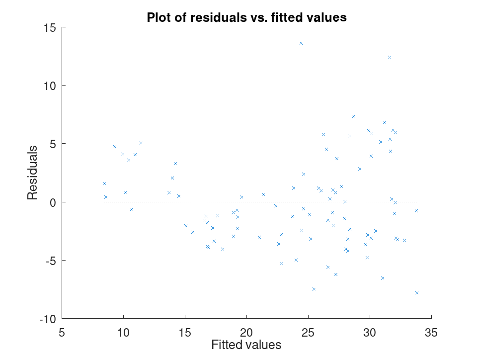
Checking residuals against fitted values. We fit a mileage model on the carsmall data set using weight and horsepower, then plot the raw residuals against the fitted values. A pattern in this plot, rather than a random scatter, would suggest the linear model is missing some curvature in the relationship.
 load carsmall
 X = [Weight, Horsepower];
 y = MPG;
 mdl = fitlm (X, y);
 plotResiduals (mdl, 'fitted')
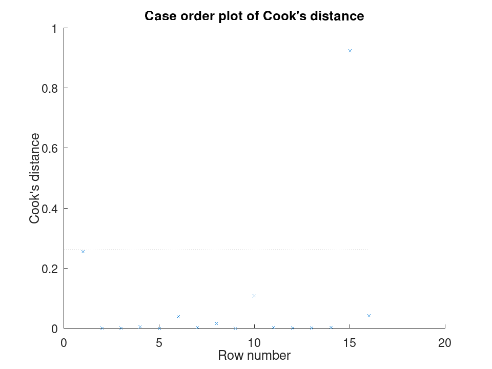
Spotting influential observations with Cook's distance. Sixteen houses are matched by size and age to a sale price, but one house was sold far above what its size and age would predict. After fitting the model, plotDiagnostics with the cookd option highlights that single observation as having outsized influence on the fit.
 Size  = [80; 95; 110; 120; 65; 140; 100; 130; 90; 150; 75; 105; ...
          115; 85; 135; 125];
 Age   = [5; 10; 3; 8; 20; 2; 15; 6; 12; 1; 18; 9; 4; 14; 7; 11];
 Price = [200; 230; 260; 280; 150; 320; 240; 300; 210; 340; 170; ...
          250; 270; 190; 500; 290];
 X = [Size, Age];
 y = Price;
 mdl = fitlm (X, y);
 plotDiagnostics (mdl, 'cookd')
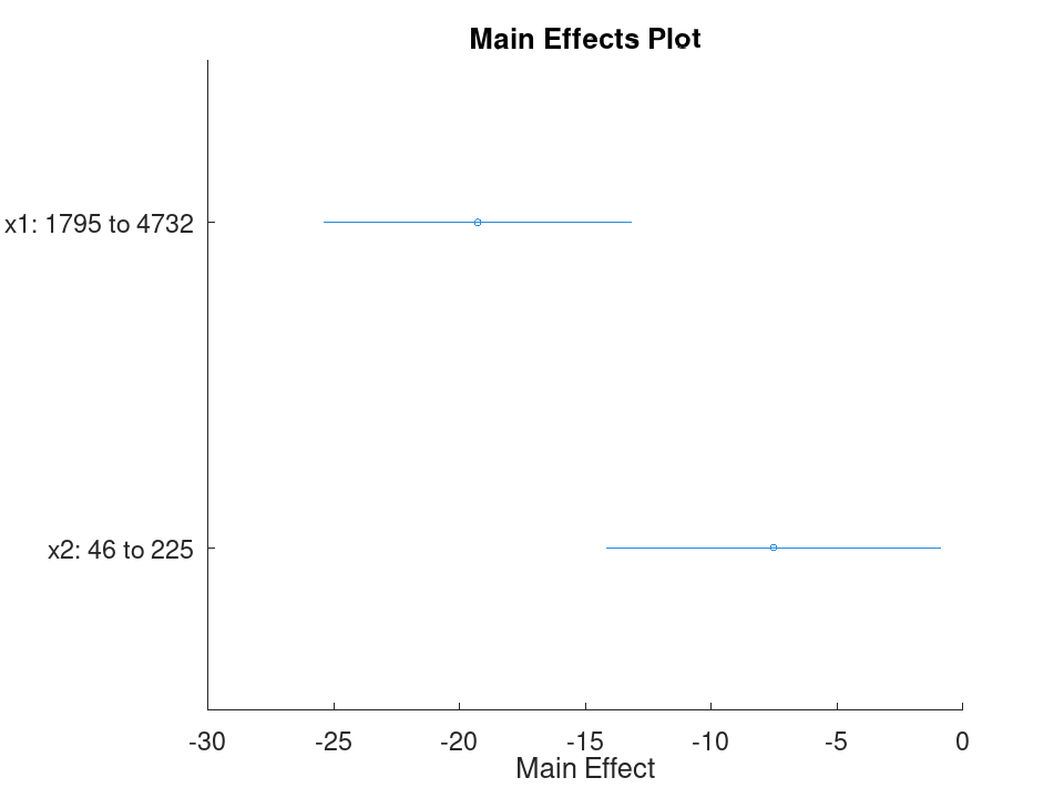
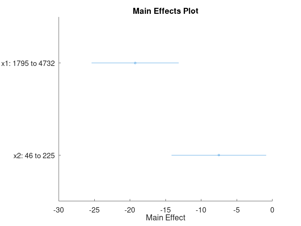
Comparing the size of each predictor's effect, alongside a hypothesis test on the model as a whole. We fit a mileage model on the carsmall data set using weight and horsepower. plotEffects draws each coefficient's estimate with its confidence interval side by side, and coefTest checks whether weight's effect is significantly different from horsepower's.
 load carsmall
 X = [Weight, Horsepower];
 y = MPG;
 mdl = fitlm (X, y);
Visualize the relative size of each predictor's effect.
plotEffects (mdl)
Test whether the two coefficients differ significantly.
 H = [0 1 -1];
 [p, F, r] = coefTest (mdl, H)
p = 0.073643
F = 3.2759
r = 1
A positive integer equal to the number of observations minus the number
of estimated coefficients: DFE = NumObservations -
NumEstimatedCoefficients. This property is read-only.
Simple linear regression with a single predictor. Ten runners record their weekly training distance and their finish time in a 10k race. We fit a straight line through this data and look at the fitted coefficients, then use predict to estimate the finish time for a runner who trains a distance not in the sample.
 Distance = [10; 15; 20; 25; 30; 35; 40; 45; 50; 55];
 Time     = [58; 55; 52; 50; 47; 45; 43; 41; 40; 38];
 X = Distance;
 y = Time;
Fit the model and inspect the estimated slope and intercept.
mdl = fitlm (X, y)
mdl =

  Linear regression model:
      y ~ 1 + x1

  Estimated Coefficients:

  2x4 table

                   Estimate       SE         tStat        pValue
                   ________    _________    ________    ___________

    (Intercept)        61.2     0.654588      93.494    1.91213e-13
    x1                -0.44    0.0184226    -23.8836    1.00609e-08


Number of observations: 10, Error degrees of freedom: 8
Root Mean Squared Error: 0.83666
R-squared: 0.986169,  Adjusted R-Squared: 0.984441
F-statistic vs. constant model: 570.429, p-value = 1.00609e-08
Predict the finish time for a runner training 32 km per week.
ypred = predict (mdl, 32)
ypred = 47.120
Multiple linear regression with two predictors, followed by a confidence interval on the coefficients. Thirteen coffee shops report their weekly foot traffic and the number of items on their menu, along with weekly revenue. We fit a model with both predictors, then use coefCI to see how precisely each coefficient is estimated.
 Traffic = [120; 150; 90; 200; 175; 60; 220; 140; 100; 190; 80; 210; 130];
 MenuSize = [8; 12; 6; 15; 10; 5; 18; 9; 7; 14; 6; 16; 11];
 Revenue = [1450; 1820; 1010; 2400; 2050; 700; 2650; 1700; 1150; ...
            2300; 900; 2500; 1600];
 X = [Traffic, MenuSize];
 y = Revenue;
Fit the model with both predictors together.
mdl = fitlm (X, y)
mdl =

  Linear regression model:
      y ~ 1 + x1 + x2

  Estimated Coefficients:

  3x4 table

                   Estimate       SE        tStat        pValue
                   ________    ________    ________    ___________

    (Intercept)    -47.0932     27.3456    -1.72215       0.115771
    x1              11.4079    0.616078      18.517    4.55169e-09
    x2              11.4344     7.68384     1.48811       0.167562


Number of observations: 13, Error degrees of freedom: 10
Root Mean Squared Error: 32.4551
R-squared: 0.997901,  Adjusted R-Squared: 0.997482
F-statistic vs. constant model: 2377.53, p-value = 4.07061e-14
Check how tight the 95% confidence interval is on each coefficient.
ci = coefCI (mdl)
ci =

  -108.0231    13.8366
    10.0352    12.7806
    -5.6862    28.5551
Growing a model with addTerms and predicting with the richer model. We model fuel economy from the carsmall data set using weight and horsepower as main effects only. addTerms then brings in the weight-horsepower interaction without needing to refit by hand, and predict shows how the estimate for a new car changes once that interaction is included.
 load carsmall
 X = [Weight, Horsepower];
 y = MPG;
Fit the additive model first.
mdl = fitlm (X, y);
Add the interaction between weight and horsepower.
mdl2 = addTerms (mdl, 'x1:x2');
Compare predictions from both models for the same new car.
 Xnew = [3200, 120];
 ypred1 = predict (mdl, Xnew)
ypred1 = 21.719
ypred2 = predict (mdl2, Xnew)
ypred2 = 20.416
Simplifying a model with removeTerms and comparing fit quality. We fit the full Hald cement model with all four ingredients, then use removeTerms to drop the weakest predictor and refit automatically. Comparing SSE before and after shows how little explanatory power that ingredient was actually contributing.
 load hald
 X = ingredients;
 y = heat;
Fit the model with all four ingredients.
mdl = fitlm (X, y);
Drop the third ingredient and refit on the same data.
mdl2 = removeTerms (mdl, 'x3');
Compare how much the error sum of squares changed.
sse_full = mdl.SSE
sse_full = 47.864
sse_reduced = mdl2.SSE
sse_reduced = 47.973
Testing a linear hypothesis and checking residual autocorrelation. Twelve patients are given a drug at different doses over different treatment durations, and a recovery score is recorded. coefTest checks whether the dose and duration coefficients are actually equal, and dwtest separately checks whether the residuals still carry a leftover pattern the model failed to capture.
 Dose     = [10; 15; 20; 25; 30; 35; 12; 18; 22; 28; 32; 38];
 Duration = [5; 7; 9; 11; 13; 15; 6; 8; 10; 12; 14; 16];
 Recovery = [42; 48; 55; 60; 68; 74; 45; 52; 58; 65; 71; 78];
 X = [Dose, Duration];
 y = Recovery;
 mdl = fitlm (X, y);
Test H0: the Dose and Duration coefficients are equal.
 H = [0 1 -1];
 [p, F, r] = coefTest (mdl, H)
p = 0.3535
F = 0.9571
r = 1
Check for autocorrelation left over in the residuals.
[pdw, dw] = dwtest (mdl)
pdw = 0.3658
dw = 2.4432
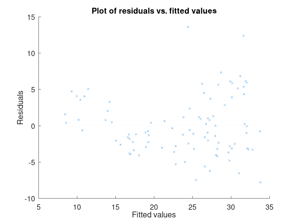
Checking residuals against fitted values. We fit a mileage model on the carsmall data set using weight and horsepower, then plot the raw residuals against the fitted values. A pattern in this plot, rather than a random scatter, would suggest the linear model is missing some curvature in the relationship.
 load carsmall
 X = [Weight, Horsepower];
 y = MPG;
 mdl = fitlm (X, y);
 plotResiduals (mdl, 'fitted')
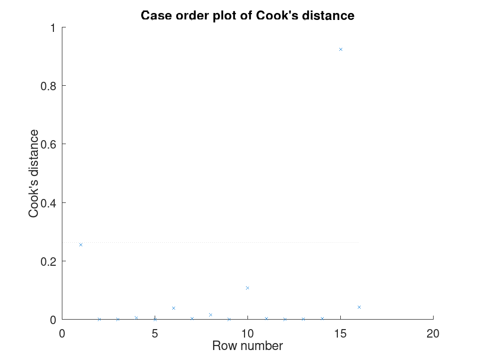
Spotting influential observations with Cook's distance. Sixteen houses are matched by size and age to a sale price, but one house was sold far above what its size and age would predict. After fitting the model, plotDiagnostics with the cookd option highlights that single observation as having outsized influence on the fit.
 Size  = [80; 95; 110; 120; 65; 140; 100; 130; 90; 150; 75; 105; ...
          115; 85; 135; 125];
 Age   = [5; 10; 3; 8; 20; 2; 15; 6; 12; 1; 18; 9; 4; 14; 7; 11];
 Price = [200; 230; 260; 280; 150; 320; 240; 300; 210; 340; 170; ...
          250; 270; 190; 500; 290];
 X = [Size, Age];
 y = Price;
 mdl = fitlm (X, y);
 plotDiagnostics (mdl, 'cookd')
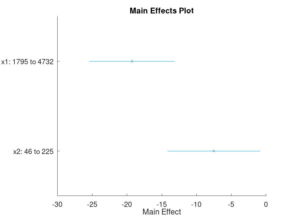
Comparing the size of each predictor's effect, alongside a hypothesis test on the model as a whole. We fit a mileage model on the carsmall data set using weight and horsepower. plotEffects draws each coefficient's estimate with its confidence interval side by side, and coefTest checks whether weight's effect is significantly different from horsepower's.
 load carsmall
 X = [Weight, Horsepower];
 y = MPG;
 mdl = fitlm (X, y);
Visualize the relative size of each predictor's effect.
plotEffects (mdl)
Test whether the two coefficients differ significantly.
 H = [0 1 -1];
 [p, F, r] = coefTest (mdl, H)
p = 0.073643
F = 3.2759
r = 1
A table with one row per observation and seven columns:
-
Leverage- diagonal of the hat matrix H -
CooksDistance- Cook’s distance, a measure of scaled change in fitted values -
Dffits- delete-1 scaled differences in fitted values -
S2_i- delete-1 residual variance estimate -
CovRatio- ratio of the determinant of the coefficient covariance matrix with and without each observation -
Dfbetas- n-by-p matrix of scaled changes in coefficient estimates when each observation is deleted in turn -
HatMatrix- n-by-n projection matrix such thatFitted = HatMatrix * y
Rows not used in fitting have NaN in CooksDistance,
Dffits, S2_i, and CovRatio, and zeros in
Leverage, Dfbetas, and HatMatrix. This property
is read-only.
Simple linear regression with a single predictor. Ten runners record their weekly training distance and their finish time in a 10k race. We fit a straight line through this data and look at the fitted coefficients, then use predict to estimate the finish time for a runner who trains a distance not in the sample.
 Distance = [10; 15; 20; 25; 30; 35; 40; 45; 50; 55];
 Time     = [58; 55; 52; 50; 47; 45; 43; 41; 40; 38];
 X = Distance;
 y = Time;
Fit the model and inspect the estimated slope and intercept.
mdl = fitlm (X, y)
mdl =

  Linear regression model:
      y ~ 1 + x1

  Estimated Coefficients:

  2x4 table

                   Estimate       SE         tStat        pValue
                   ________    _________    ________    ___________

    (Intercept)        61.2     0.654588      93.494    1.91213e-13
    x1                -0.44    0.0184226    -23.8836    1.00609e-08


Number of observations: 10, Error degrees of freedom: 8
Root Mean Squared Error: 0.83666
R-squared: 0.986169,  Adjusted R-Squared: 0.984441
F-statistic vs. constant model: 570.429, p-value = 1.00609e-08
Predict the finish time for a runner training 32 km per week.
ypred = predict (mdl, 32)
ypred = 47.120
Multiple linear regression with two predictors, followed by a confidence interval on the coefficients. Thirteen coffee shops report their weekly foot traffic and the number of items on their menu, along with weekly revenue. We fit a model with both predictors, then use coefCI to see how precisely each coefficient is estimated.
 Traffic = [120; 150; 90; 200; 175; 60; 220; 140; 100; 190; 80; 210; 130];
 MenuSize = [8; 12; 6; 15; 10; 5; 18; 9; 7; 14; 6; 16; 11];
 Revenue = [1450; 1820; 1010; 2400; 2050; 700; 2650; 1700; 1150; ...
            2300; 900; 2500; 1600];
 X = [Traffic, MenuSize];
 y = Revenue;
Fit the model with both predictors together.
mdl = fitlm (X, y)
mdl =

  Linear regression model:
      y ~ 1 + x1 + x2

  Estimated Coefficients:

  3x4 table

                   Estimate       SE        tStat        pValue
                   ________    ________    ________    ___________

    (Intercept)    -47.0932     27.3456    -1.72215       0.115771
    x1              11.4079    0.616078      18.517    4.55169e-09
    x2              11.4344     7.68384     1.48811       0.167562


Number of observations: 13, Error degrees of freedom: 10
Root Mean Squared Error: 32.4551
R-squared: 0.997901,  Adjusted R-Squared: 0.997482
F-statistic vs. constant model: 2377.53, p-value = 4.07061e-14
Check how tight the 95% confidence interval is on each coefficient.
ci = coefCI (mdl)
ci =

  -108.0231    13.8366
    10.0352    12.7806
    -5.6862    28.5551
Growing a model with addTerms and predicting with the richer model. We model fuel economy from the carsmall data set using weight and horsepower as main effects only. addTerms then brings in the weight-horsepower interaction without needing to refit by hand, and predict shows how the estimate for a new car changes once that interaction is included.
 load carsmall
 X = [Weight, Horsepower];
 y = MPG;
Fit the additive model first.
mdl = fitlm (X, y);
Add the interaction between weight and horsepower.
mdl2 = addTerms (mdl, 'x1:x2');
Compare predictions from both models for the same new car.
 Xnew = [3200, 120];
 ypred1 = predict (mdl, Xnew)
ypred1 = 21.719
ypred2 = predict (mdl2, Xnew)
ypred2 = 20.416
Simplifying a model with removeTerms and comparing fit quality. We fit the full Hald cement model with all four ingredients, then use removeTerms to drop the weakest predictor and refit automatically. Comparing SSE before and after shows how little explanatory power that ingredient was actually contributing.
 load hald
 X = ingredients;
 y = heat;
Fit the model with all four ingredients.
mdl = fitlm (X, y);
Drop the third ingredient and refit on the same data.
mdl2 = removeTerms (mdl, 'x3');
Compare how much the error sum of squares changed.
sse_full = mdl.SSE
sse_full = 47.864
sse_reduced = mdl2.SSE
sse_reduced = 47.973
Testing a linear hypothesis and checking residual autocorrelation. Twelve patients are given a drug at different doses over different treatment durations, and a recovery score is recorded. coefTest checks whether the dose and duration coefficients are actually equal, and dwtest separately checks whether the residuals still carry a leftover pattern the model failed to capture.
 Dose     = [10; 15; 20; 25; 30; 35; 12; 18; 22; 28; 32; 38];
 Duration = [5; 7; 9; 11; 13; 15; 6; 8; 10; 12; 14; 16];
 Recovery = [42; 48; 55; 60; 68; 74; 45; 52; 58; 65; 71; 78];
 X = [Dose, Duration];
 y = Recovery;
 mdl = fitlm (X, y);
Test H0: the Dose and Duration coefficients are equal.
 H = [0 1 -1];
 [p, F, r] = coefTest (mdl, H)
p = 0.3535
F = 0.9571
r = 1
Check for autocorrelation left over in the residuals.
[pdw, dw] = dwtest (mdl)
pdw = 0.3658
dw = 2.4432
Checking residuals against fitted values. We fit a mileage model on the carsmall data set using weight and horsepower, then plot the raw residuals against the fitted values. A pattern in this plot, rather than a random scatter, would suggest the linear model is missing some curvature in the relationship.
 load carsmall
 X = [Weight, Horsepower];
 y = MPG;
 mdl = fitlm (X, y);
 plotResiduals (mdl, 'fitted')
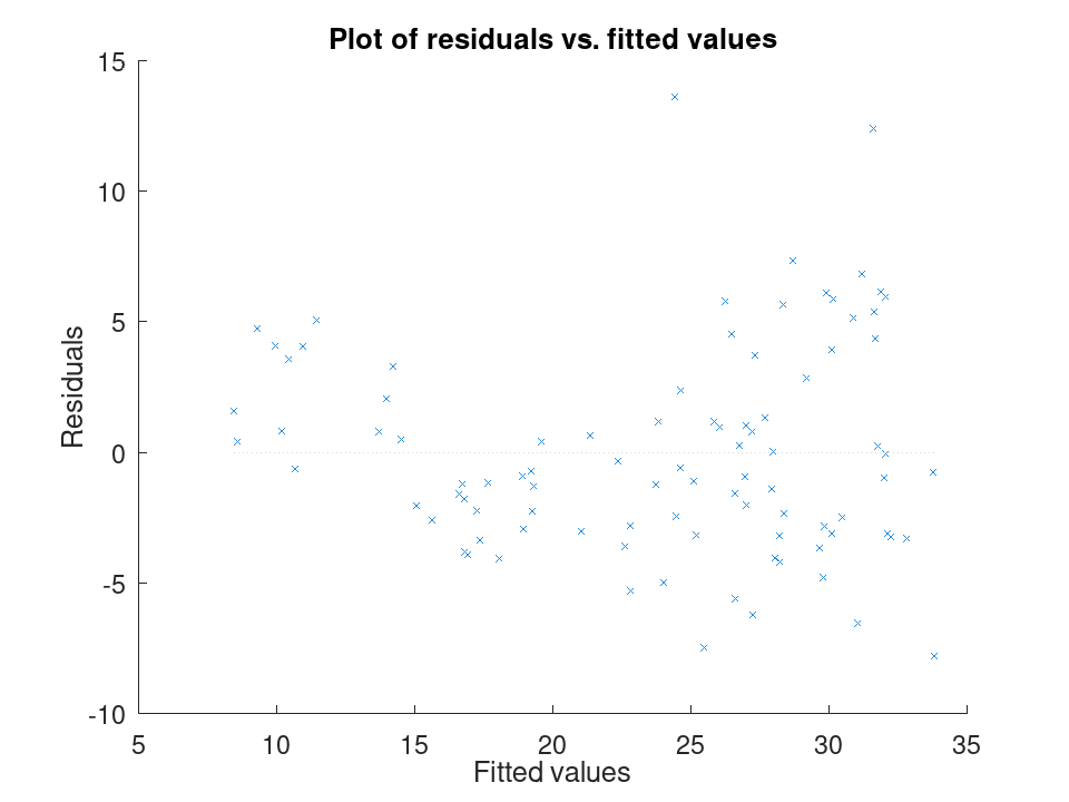
Spotting influential observations with Cook's distance. Sixteen houses are matched by size and age to a sale price, but one house was sold far above what its size and age would predict. After fitting the model, plotDiagnostics with the cookd option highlights that single observation as having outsized influence on the fit.
 Size  = [80; 95; 110; 120; 65; 140; 100; 130; 90; 150; 75; 105; ...
          115; 85; 135; 125];
 Age   = [5; 10; 3; 8; 20; 2; 15; 6; 12; 1; 18; 9; 4; 14; 7; 11];
 Price = [200; 230; 260; 280; 150; 320; 240; 300; 210; 340; 170; ...
          250; 270; 190; 500; 290];
 X = [Size, Age];
 y = Price;
 mdl = fitlm (X, y);
 plotDiagnostics (mdl, 'cookd')
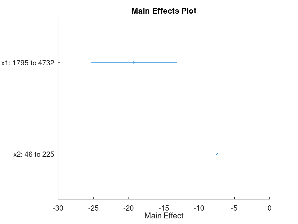
Comparing the size of each predictor's effect, alongside a hypothesis test on the model as a whole. We fit a mileage model on the carsmall data set using weight and horsepower. plotEffects draws each coefficient's estimate with its confidence interval side by side, and coefTest checks whether weight's effect is significantly different from horsepower's.
 load carsmall
 X = [Weight, Horsepower];
 y = MPG;
 mdl = fitlm (X, y);
Visualize the relative size of each predictor's effect.
plotEffects (mdl)
Test whether the two coefficients differ significantly.
 H = [0 1 -1];
 [p, F, r] = coefTest (mdl, H)
p = 0.073643
F = 3.2759
r = 1
An n-by-1 numeric vector of predicted response values based on
the training data, where n is the total number of observations,
excluded and missing rows included. Every observation whose predictors
are available carries a fitted value, whether or not it was used in the
fit, so an excluded row and a row missing only its response are both
fitted; only a row whose predictors are missing is NaN. The
corresponding Residuals are NaN for any row not used in
the fit, so Fitted and Residuals.Raw do not add back to
the response there. Use predict to obtain predictions for new
data or to compute confidence bounds. This property is read-only.
Simple linear regression with a single predictor. Ten runners record their weekly training distance and their finish time in a 10k race. We fit a straight line through this data and look at the fitted coefficients, then use predict to estimate the finish time for a runner who trains a distance not in the sample.
 Distance = [10; 15; 20; 25; 30; 35; 40; 45; 50; 55];
 Time     = [58; 55; 52; 50; 47; 45; 43; 41; 40; 38];
 X = Distance;
 y = Time;
Fit the model and inspect the estimated slope and intercept.
mdl = fitlm (X, y)
mdl =

  Linear regression model:
      y ~ 1 + x1

  Estimated Coefficients:

  2x4 table

                   Estimate       SE         tStat        pValue
                   ________    _________    ________    ___________

    (Intercept)        61.2     0.654588      93.494    1.91213e-13
    x1                -0.44    0.0184226    -23.8836    1.00609e-08


Number of observations: 10, Error degrees of freedom: 8
Root Mean Squared Error: 0.83666
R-squared: 0.986169,  Adjusted R-Squared: 0.984441
F-statistic vs. constant model: 570.429, p-value = 1.00609e-08
Predict the finish time for a runner training 32 km per week.
ypred = predict (mdl, 32)
ypred = 47.120
Multiple linear regression with two predictors, followed by a confidence interval on the coefficients. Thirteen coffee shops report their weekly foot traffic and the number of items on their menu, along with weekly revenue. We fit a model with both predictors, then use coefCI to see how precisely each coefficient is estimated.
 Traffic = [120; 150; 90; 200; 175; 60; 220; 140; 100; 190; 80; 210; 130];
 MenuSize = [8; 12; 6; 15; 10; 5; 18; 9; 7; 14; 6; 16; 11];
 Revenue = [1450; 1820; 1010; 2400; 2050; 700; 2650; 1700; 1150; ...
            2300; 900; 2500; 1600];
 X = [Traffic, MenuSize];
 y = Revenue;
Fit the model with both predictors together.
mdl = fitlm (X, y)
mdl =

  Linear regression model:
      y ~ 1 + x1 + x2

  Estimated Coefficients:

  3x4 table

                   Estimate       SE        tStat        pValue
                   ________    ________    ________    ___________

    (Intercept)    -47.0932     27.3456    -1.72215       0.115771
    x1              11.4079    0.616078      18.517    4.55169e-09
    x2              11.4344     7.68384     1.48811       0.167562


Number of observations: 13, Error degrees of freedom: 10
Root Mean Squared Error: 32.4551
R-squared: 0.997901,  Adjusted R-Squared: 0.997482
F-statistic vs. constant model: 2377.53, p-value = 4.07061e-14
Check how tight the 95% confidence interval is on each coefficient.
ci = coefCI (mdl)
ci =

  -108.0231    13.8366
    10.0352    12.7806
    -5.6862    28.5551
Growing a model with addTerms and predicting with the richer model. We model fuel economy from the carsmall data set using weight and horsepower as main effects only. addTerms then brings in the weight-horsepower interaction without needing to refit by hand, and predict shows how the estimate for a new car changes once that interaction is included.
 load carsmall
 X = [Weight, Horsepower];
 y = MPG;
Fit the additive model first.
mdl = fitlm (X, y);
Add the interaction between weight and horsepower.
mdl2 = addTerms (mdl, 'x1:x2');
Compare predictions from both models for the same new car.
 Xnew = [3200, 120];
 ypred1 = predict (mdl, Xnew)
ypred1 = 21.719
ypred2 = predict (mdl2, Xnew)
ypred2 = 20.416
Simplifying a model with removeTerms and comparing fit quality. We fit the full Hald cement model with all four ingredients, then use removeTerms to drop the weakest predictor and refit automatically. Comparing SSE before and after shows how little explanatory power that ingredient was actually contributing.
 load hald
 X = ingredients;
 y = heat;
Fit the model with all four ingredients.
mdl = fitlm (X, y);
Drop the third ingredient and refit on the same data.
mdl2 = removeTerms (mdl, 'x3');
Compare how much the error sum of squares changed.
sse_full = mdl.SSE
sse_full = 47.864
sse_reduced = mdl2.SSE
sse_reduced = 47.973
Testing a linear hypothesis and checking residual autocorrelation. Twelve patients are given a drug at different doses over different treatment durations, and a recovery score is recorded. coefTest checks whether the dose and duration coefficients are actually equal, and dwtest separately checks whether the residuals still carry a leftover pattern the model failed to capture.
 Dose     = [10; 15; 20; 25; 30; 35; 12; 18; 22; 28; 32; 38];
 Duration = [5; 7; 9; 11; 13; 15; 6; 8; 10; 12; 14; 16];
 Recovery = [42; 48; 55; 60; 68; 74; 45; 52; 58; 65; 71; 78];
 X = [Dose, Duration];
 y = Recovery;
 mdl = fitlm (X, y);
Test H0: the Dose and Duration coefficients are equal.
 H = [0 1 -1];
 [p, F, r] = coefTest (mdl, H)
p = 0.3535
F = 0.9571
r = 1
Check for autocorrelation left over in the residuals.
[pdw, dw] = dwtest (mdl)
pdw = 0.3658
dw = 2.4432
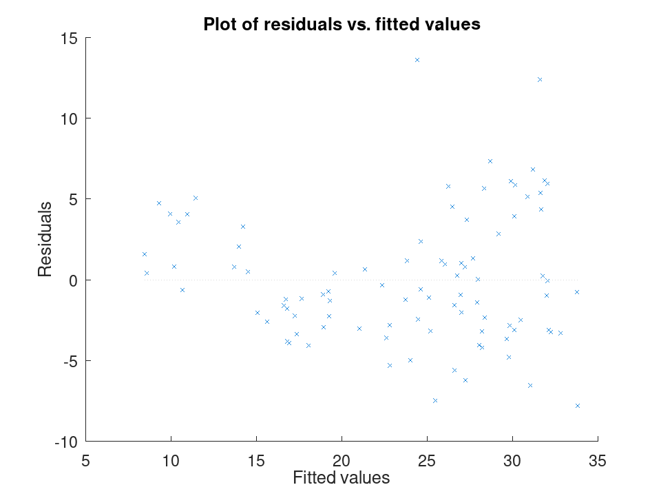
Checking residuals against fitted values. We fit a mileage model on the carsmall data set using weight and horsepower, then plot the raw residuals against the fitted values. A pattern in this plot, rather than a random scatter, would suggest the linear model is missing some curvature in the relationship.
 load carsmall
 X = [Weight, Horsepower];
 y = MPG;
 mdl = fitlm (X, y);
 plotResiduals (mdl, 'fitted')
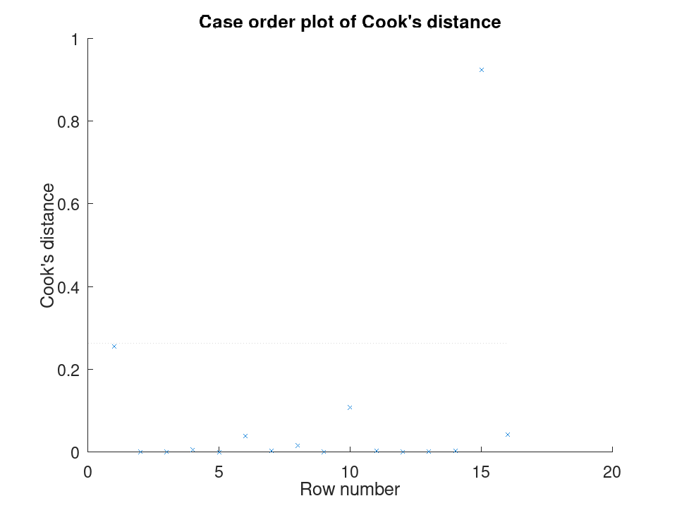
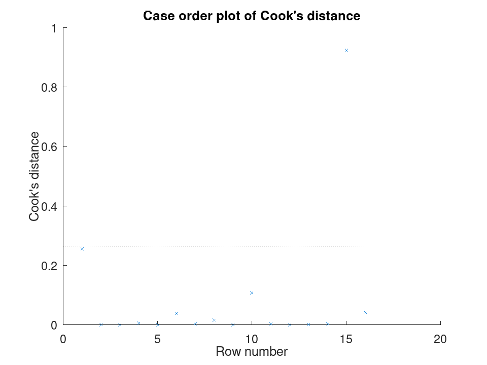
Spotting influential observations with Cook's distance. Sixteen houses are matched by size and age to a sale price, but one house was sold far above what its size and age would predict. After fitting the model, plotDiagnostics with the cookd option highlights that single observation as having outsized influence on the fit.
 Size  = [80; 95; 110; 120; 65; 140; 100; 130; 90; 150; 75; 105; ...
          115; 85; 135; 125];
 Age   = [5; 10; 3; 8; 20; 2; 15; 6; 12; 1; 18; 9; 4; 14; 7; 11];
 Price = [200; 230; 260; 280; 150; 320; 240; 300; 210; 340; 170; ...
          250; 270; 190; 500; 290];
 X = [Size, Age];
 y = Price;
 mdl = fitlm (X, y);
 plotDiagnostics (mdl, 'cookd')
Comparing the size of each predictor's effect, alongside a hypothesis test on the model as a whole. We fit a mileage model on the carsmall data set using weight and horsepower. plotEffects draws each coefficient's estimate with its confidence interval side by side, and coefTest checks whether weight's effect is significantly different from horsepower's.
 load carsmall
 X = [Weight, Horsepower];
 y = MPG;
 mdl = fitlm (X, y);
Visualize the relative size of each predictor's effect.
plotEffects (mdl)
Test whether the two coefficients differ significantly.
 H = [0 1 -1];
 [p, F, r] = coefTest (mdl, H)
p = 0.073643
F = 3.2759
r = 1
A scalar numeric value equal to the log-likelihood of the response values, assuming each response is normally distributed with mean equal to the fitted value and variance equal to SSE/n (the MLE variance estimate). This property is read-only.
For a weighted fit, observation i is taken to have variance s^2/w_i, so the log-likelihood carries the term 0.5 × sum (log (w)) and n counts only the observations with nonzero weight:
logL = -n/2 × (1 + log (2×pi×SSE/n)) + 0.5 × sum (log (w))
This makes the value invariant to the scale of the weights, as it must be: multiplying every weight by a constant rescales the estimated variance by the same constant and leaves the fit unchanged.
MATLAB omits the 0.5 × sum (log (w)) term and counts every
observation in n, so its LogLikelihood moves by
n/2 × log (c) when the weights are multiplied by c, and
the ModelCriterion values built on it move with it. This
implementation follows R’s logLik.lm instead. Unweighted fits
are unaffected, and agree with MATLAB.
A robust fit carries no weight term. Its SSE is a robust scale
estimate rather than a weighted residual sum, so the two enter
separately and the general form is used:
logL = -n/2 × log (2×pi×SSE/n) - sum (w .× r.^2) / (2×SSE/n)
which is what MATLAB computes, and which reduces to the expression
above whenever sum (w .× r.^2) equals SSE, as it does for
any least-squares fit. Robust fits therefore agree with MATLAB
exactly, weighted or not.
Simple linear regression with a single predictor. Ten runners record their weekly training distance and their finish time in a 10k race. We fit a straight line through this data and look at the fitted coefficients, then use predict to estimate the finish time for a runner who trains a distance not in the sample.
 Distance = [10; 15; 20; 25; 30; 35; 40; 45; 50; 55];
 Time     = [58; 55; 52; 50; 47; 45; 43; 41; 40; 38];
 X = Distance;
 y = Time;
Fit the model and inspect the estimated slope and intercept.
mdl = fitlm (X, y)
mdl =

  Linear regression model:
      y ~ 1 + x1

  Estimated Coefficients:

  2x4 table

                   Estimate       SE         tStat        pValue
                   ________    _________    ________    ___________

    (Intercept)        61.2     0.654588      93.494    1.91213e-13
    x1                -0.44    0.0184226    -23.8836    1.00609e-08


Number of observations: 10, Error degrees of freedom: 8
Root Mean Squared Error: 0.83666
R-squared: 0.986169,  Adjusted R-Squared: 0.984441
F-statistic vs. constant model: 570.429, p-value = 1.00609e-08
Predict the finish time for a runner training 32 km per week.
ypred = predict (mdl, 32)
ypred = 47.120
Multiple linear regression with two predictors, followed by a confidence interval on the coefficients. Thirteen coffee shops report their weekly foot traffic and the number of items on their menu, along with weekly revenue. We fit a model with both predictors, then use coefCI to see how precisely each coefficient is estimated.
 Traffic = [120; 150; 90; 200; 175; 60; 220; 140; 100; 190; 80; 210; 130];
 MenuSize = [8; 12; 6; 15; 10; 5; 18; 9; 7; 14; 6; 16; 11];
 Revenue = [1450; 1820; 1010; 2400; 2050; 700; 2650; 1700; 1150; ...
            2300; 900; 2500; 1600];
 X = [Traffic, MenuSize];
 y = Revenue;
Fit the model with both predictors together.
mdl = fitlm (X, y)
mdl =

  Linear regression model:
      y ~ 1 + x1 + x2

  Estimated Coefficients:

  3x4 table

                   Estimate       SE        tStat        pValue
                   ________    ________    ________    ___________

    (Intercept)    -47.0932     27.3456    -1.72215       0.115771
    x1              11.4079    0.616078      18.517    4.55169e-09
    x2              11.4344     7.68384     1.48811       0.167562


Number of observations: 13, Error degrees of freedom: 10
Root Mean Squared Error: 32.4551
R-squared: 0.997901,  Adjusted R-Squared: 0.997482
F-statistic vs. constant model: 2377.53, p-value = 4.07061e-14
Check how tight the 95% confidence interval is on each coefficient.
ci = coefCI (mdl)
ci =

  -108.0231    13.8366
    10.0352    12.7806
    -5.6862    28.5551
Growing a model with addTerms and predicting with the richer model. We model fuel economy from the carsmall data set using weight and horsepower as main effects only. addTerms then brings in the weight-horsepower interaction without needing to refit by hand, and predict shows how the estimate for a new car changes once that interaction is included.
 load carsmall
 X = [Weight, Horsepower];
 y = MPG;
Fit the additive model first.
mdl = fitlm (X, y);
Add the interaction between weight and horsepower.
mdl2 = addTerms (mdl, 'x1:x2');
Compare predictions from both models for the same new car.
 Xnew = [3200, 120];
 ypred1 = predict (mdl, Xnew)
ypred1 = 21.719
ypred2 = predict (mdl2, Xnew)
ypred2 = 20.416
Simplifying a model with removeTerms and comparing fit quality. We fit the full Hald cement model with all four ingredients, then use removeTerms to drop the weakest predictor and refit automatically. Comparing SSE before and after shows how little explanatory power that ingredient was actually contributing.
 load hald
 X = ingredients;
 y = heat;
Fit the model with all four ingredients.
mdl = fitlm (X, y);
Drop the third ingredient and refit on the same data.
mdl2 = removeTerms (mdl, 'x3');
Compare how much the error sum of squares changed.
sse_full = mdl.SSE
sse_full = 47.864
sse_reduced = mdl2.SSE
sse_reduced = 47.973
Testing a linear hypothesis and checking residual autocorrelation. Twelve patients are given a drug at different doses over different treatment durations, and a recovery score is recorded. coefTest checks whether the dose and duration coefficients are actually equal, and dwtest separately checks whether the residuals still carry a leftover pattern the model failed to capture.
 Dose     = [10; 15; 20; 25; 30; 35; 12; 18; 22; 28; 32; 38];
 Duration = [5; 7; 9; 11; 13; 15; 6; 8; 10; 12; 14; 16];
 Recovery = [42; 48; 55; 60; 68; 74; 45; 52; 58; 65; 71; 78];
 X = [Dose, Duration];
 y = Recovery;
 mdl = fitlm (X, y);
Test H0: the Dose and Duration coefficients are equal.
 H = [0 1 -1];
 [p, F, r] = coefTest (mdl, H)
p = 0.3535
F = 0.9571
r = 1
Check for autocorrelation left over in the residuals.
[pdw, dw] = dwtest (mdl)
pdw = 0.3658
dw = 2.4432
Checking residuals against fitted values. We fit a mileage model on the carsmall data set using weight and horsepower, then plot the raw residuals against the fitted values. A pattern in this plot, rather than a random scatter, would suggest the linear model is missing some curvature in the relationship.
 load carsmall
 X = [Weight, Horsepower];
 y = MPG;
 mdl = fitlm (X, y);
 plotResiduals (mdl, 'fitted')
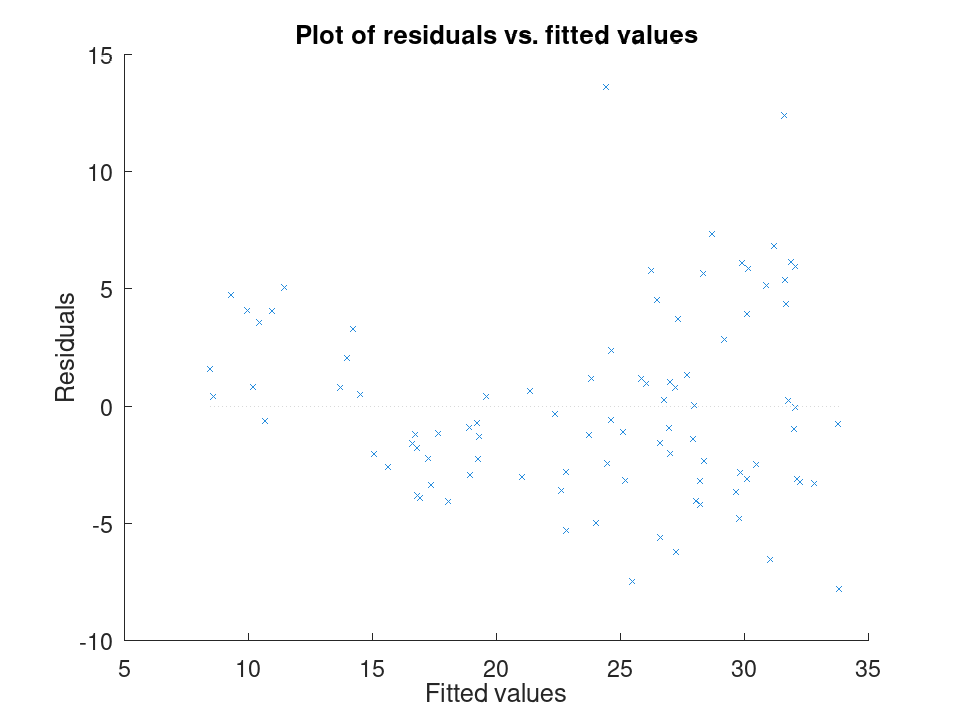
Spotting influential observations with Cook's distance. Sixteen houses are matched by size and age to a sale price, but one house was sold far above what its size and age would predict. After fitting the model, plotDiagnostics with the cookd option highlights that single observation as having outsized influence on the fit.
 Size  = [80; 95; 110; 120; 65; 140; 100; 130; 90; 150; 75; 105; ...
          115; 85; 135; 125];
 Age   = [5; 10; 3; 8; 20; 2; 15; 6; 12; 1; 18; 9; 4; 14; 7; 11];
 Price = [200; 230; 260; 280; 150; 320; 240; 300; 210; 340; 170; ...
          250; 270; 190; 500; 290];
 X = [Size, Age];
 y = Price;
 mdl = fitlm (X, y);
 plotDiagnostics (mdl, 'cookd')
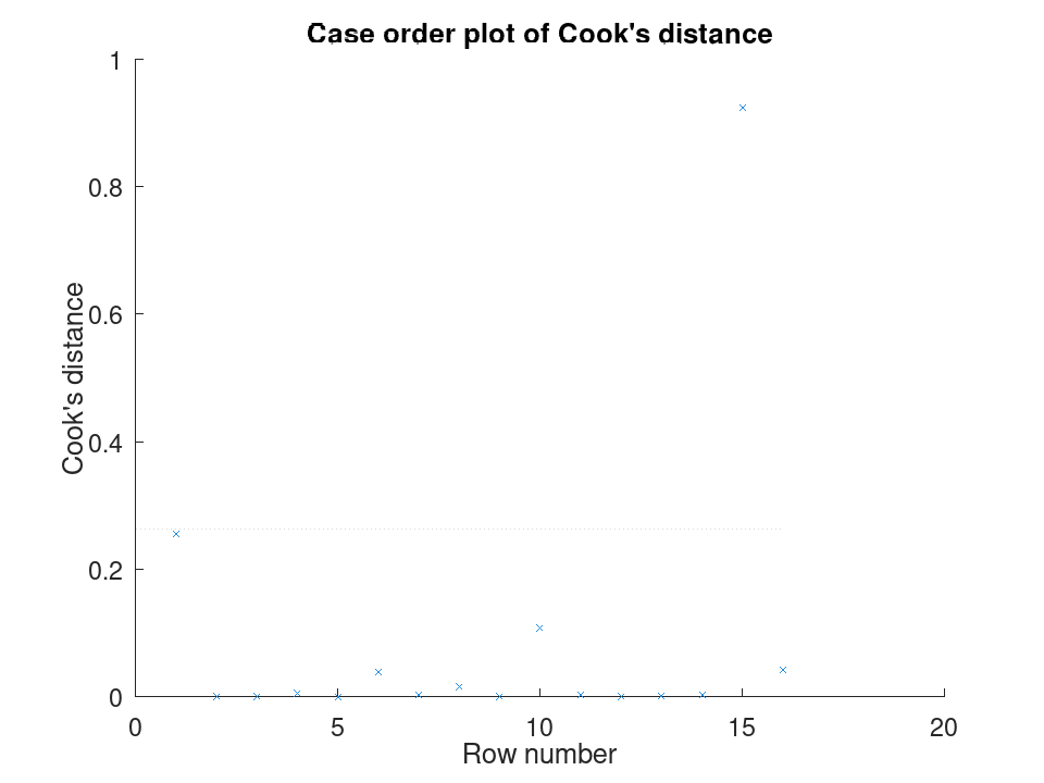
Comparing the size of each predictor's effect, alongside a hypothesis test on the model as a whole. We fit a mileage model on the carsmall data set using weight and horsepower. plotEffects draws each coefficient's estimate with its confidence interval side by side, and coefTest checks whether weight's effect is significantly different from horsepower's.
 load carsmall
 X = [Weight, Horsepower];
 y = MPG;
 mdl = fitlm (X, y);
Visualize the relative size of each predictor's effect.
plotEffects (mdl)
Test whether the two coefficients differ significantly.
 H = [0 1 -1];
 [p, F, r] = coefTest (mdl, H)
p = 0.073643
F = 3.2759
r = 1
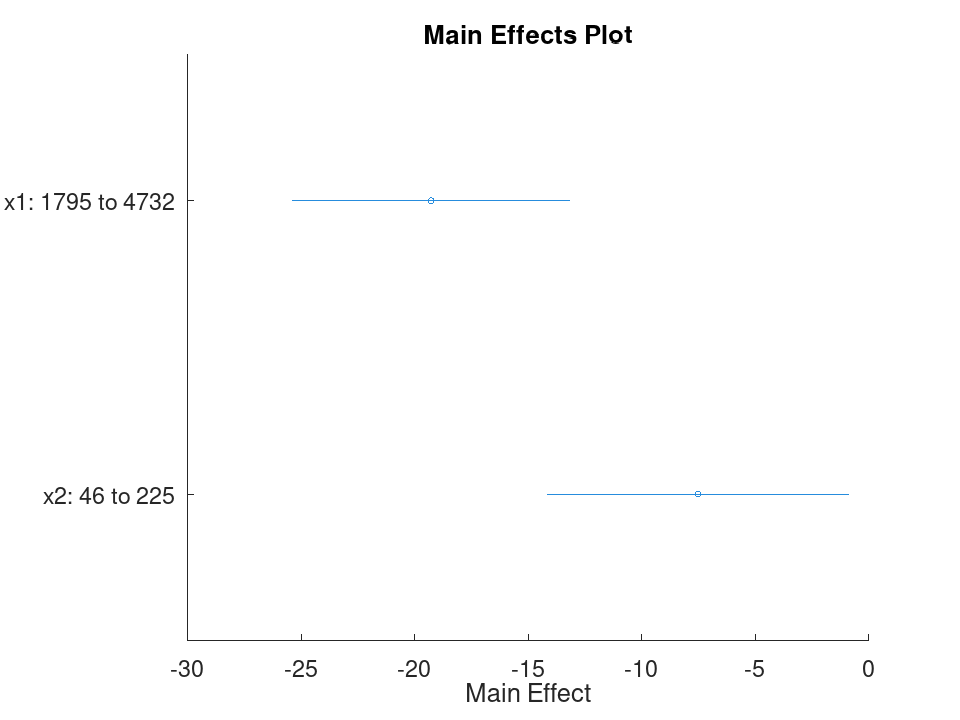
A structure with four fields:
-
AIC- Akaike information criterion: -2 × logL + 2 × m -
AICc- AIC corrected for sample size: AIC + (2×m×(m+1))/(n-m-1) -
BIC- Bayesian information criterion: -2 × logL + m × log(n) -
CAIC- Consistent AIC: -2 × logL + m × (log(n) + 1)
Here logL is LogLikelihood, m is
NumEstimatedCoefficients, and n is the number of
observations with nonzero weight, which is NumObservations
unless some weight is zero. This property is read-only.
Because these are built on LogLikelihood, they inherit its
treatment of weights; see that property for how it differs from
MATLAB’s.
Simple linear regression with a single predictor. Ten runners record their weekly training distance and their finish time in a 10k race. We fit a straight line through this data and look at the fitted coefficients, then use predict to estimate the finish time for a runner who trains a distance not in the sample.
 Distance = [10; 15; 20; 25; 30; 35; 40; 45; 50; 55];
 Time     = [58; 55; 52; 50; 47; 45; 43; 41; 40; 38];
 X = Distance;
 y = Time;
Fit the model and inspect the estimated slope and intercept.
mdl = fitlm (X, y)
mdl =

  Linear regression model:
      y ~ 1 + x1

  Estimated Coefficients:

  2x4 table

                   Estimate       SE         tStat        pValue
                   ________    _________    ________    ___________

    (Intercept)        61.2     0.654588      93.494    1.91213e-13
    x1                -0.44    0.0184226    -23.8836    1.00609e-08


Number of observations: 10, Error degrees of freedom: 8
Root Mean Squared Error: 0.83666
R-squared: 0.986169,  Adjusted R-Squared: 0.984441
F-statistic vs. constant model: 570.429, p-value = 1.00609e-08
Predict the finish time for a runner training 32 km per week.
ypred = predict (mdl, 32)
ypred = 47.120
Multiple linear regression with two predictors, followed by a confidence interval on the coefficients. Thirteen coffee shops report their weekly foot traffic and the number of items on their menu, along with weekly revenue. We fit a model with both predictors, then use coefCI to see how precisely each coefficient is estimated.
 Traffic = [120; 150; 90; 200; 175; 60; 220; 140; 100; 190; 80; 210; 130];
 MenuSize = [8; 12; 6; 15; 10; 5; 18; 9; 7; 14; 6; 16; 11];
 Revenue = [1450; 1820; 1010; 2400; 2050; 700; 2650; 1700; 1150; ...
            2300; 900; 2500; 1600];
 X = [Traffic, MenuSize];
 y = Revenue;
Fit the model with both predictors together.
mdl = fitlm (X, y)
mdl =

  Linear regression model:
      y ~ 1 + x1 + x2

  Estimated Coefficients:

  3x4 table

                   Estimate       SE        tStat        pValue
                   ________    ________    ________    ___________

    (Intercept)    -47.0932     27.3456    -1.72215       0.115771
    x1              11.4079    0.616078      18.517    4.55169e-09
    x2              11.4344     7.68384     1.48811       0.167562


Number of observations: 13, Error degrees of freedom: 10
Root Mean Squared Error: 32.4551
R-squared: 0.997901,  Adjusted R-Squared: 0.997482
F-statistic vs. constant model: 2377.53, p-value = 4.07061e-14
Check how tight the 95% confidence interval is on each coefficient.
ci = coefCI (mdl)
ci =

  -108.0231    13.8366
    10.0352    12.7806
    -5.6862    28.5551
Growing a model with addTerms and predicting with the richer model. We model fuel economy from the carsmall data set using weight and horsepower as main effects only. addTerms then brings in the weight-horsepower interaction without needing to refit by hand, and predict shows how the estimate for a new car changes once that interaction is included.
 load carsmall
 X = [Weight, Horsepower];
 y = MPG;
Fit the additive model first.
mdl = fitlm (X, y);
Add the interaction between weight and horsepower.
mdl2 = addTerms (mdl, 'x1:x2');
Compare predictions from both models for the same new car.
 Xnew = [3200, 120];
 ypred1 = predict (mdl, Xnew)
ypred1 = 21.719
ypred2 = predict (mdl2, Xnew)
ypred2 = 20.416
Simplifying a model with removeTerms and comparing fit quality. We fit the full Hald cement model with all four ingredients, then use removeTerms to drop the weakest predictor and refit automatically. Comparing SSE before and after shows how little explanatory power that ingredient was actually contributing.
 load hald
 X = ingredients;
 y = heat;
Fit the model with all four ingredients.
mdl = fitlm (X, y);
Drop the third ingredient and refit on the same data.
mdl2 = removeTerms (mdl, 'x3');
Compare how much the error sum of squares changed.
sse_full = mdl.SSE
sse_full = 47.864
sse_reduced = mdl2.SSE
sse_reduced = 47.973
Testing a linear hypothesis and checking residual autocorrelation. Twelve patients are given a drug at different doses over different treatment durations, and a recovery score is recorded. coefTest checks whether the dose and duration coefficients are actually equal, and dwtest separately checks whether the residuals still carry a leftover pattern the model failed to capture.
 Dose     = [10; 15; 20; 25; 30; 35; 12; 18; 22; 28; 32; 38];
 Duration = [5; 7; 9; 11; 13; 15; 6; 8; 10; 12; 14; 16];
 Recovery = [42; 48; 55; 60; 68; 74; 45; 52; 58; 65; 71; 78];
 X = [Dose, Duration];
 y = Recovery;
 mdl = fitlm (X, y);
Test H0: the Dose and Duration coefficients are equal.
 H = [0 1 -1];
 [p, F, r] = coefTest (mdl, H)
p = 0.3535
F = 0.9571
r = 1
Check for autocorrelation left over in the residuals.
[pdw, dw] = dwtest (mdl)
pdw = 0.3658
dw = 2.4432
Checking residuals against fitted values. We fit a mileage model on the carsmall data set using weight and horsepower, then plot the raw residuals against the fitted values. A pattern in this plot, rather than a random scatter, would suggest the linear model is missing some curvature in the relationship.
 load carsmall
 X = [Weight, Horsepower];
 y = MPG;
 mdl = fitlm (X, y);
 plotResiduals (mdl, 'fitted')
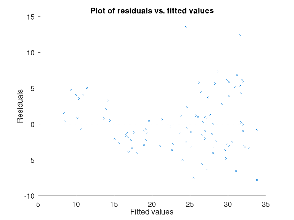
Spotting influential observations with Cook's distance. Sixteen houses are matched by size and age to a sale price, but one house was sold far above what its size and age would predict. After fitting the model, plotDiagnostics with the cookd option highlights that single observation as having outsized influence on the fit.
 Size  = [80; 95; 110; 120; 65; 140; 100; 130; 90; 150; 75; 105; ...
          115; 85; 135; 125];
 Age   = [5; 10; 3; 8; 20; 2; 15; 6; 12; 1; 18; 9; 4; 14; 7; 11];
 Price = [200; 230; 260; 280; 150; 320; 240; 300; 210; 340; 170; ...
          250; 270; 190; 500; 290];
 X = [Size, Age];
 y = Price;
 mdl = fitlm (X, y);
 plotDiagnostics (mdl, 'cookd')
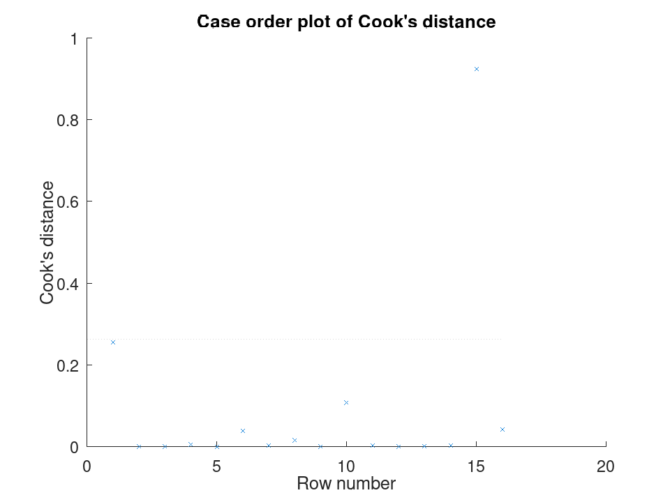
Comparing the size of each predictor's effect, alongside a hypothesis test on the model as a whole. We fit a mileage model on the carsmall data set using weight and horsepower. plotEffects draws each coefficient's estimate with its confidence interval side by side, and coefTest checks whether weight's effect is significantly different from horsepower's.
 load carsmall
 X = [Weight, Horsepower];
 y = MPG;
 mdl = fitlm (X, y);
Visualize the relative size of each predictor's effect.
plotEffects (mdl)
Test whether the two coefficients differ significantly.
 H = [0 1 -1];
 [p, F, r] = coefTest (mdl, H)
p = 0.073643
F = 3.2759
r = 1
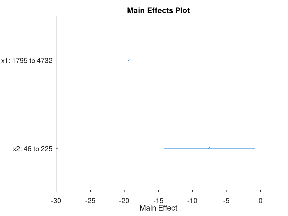
A structure with three fields:
-
Fstat- F-statistic of the fitted model versus a null model containing only a constant term -
Pvalue- p-value for the F-statistic -
NullModel- character vector describing the null model
This property is read-only.
Simple linear regression with a single predictor. Ten runners record their weekly training distance and their finish time in a 10k race. We fit a straight line through this data and look at the fitted coefficients, then use predict to estimate the finish time for a runner who trains a distance not in the sample.
 Distance = [10; 15; 20; 25; 30; 35; 40; 45; 50; 55];
 Time     = [58; 55; 52; 50; 47; 45; 43; 41; 40; 38];
 X = Distance;
 y = Time;
Fit the model and inspect the estimated slope and intercept.
mdl = fitlm (X, y)
mdl =

  Linear regression model:
      y ~ 1 + x1

  Estimated Coefficients:

  2x4 table

                   Estimate       SE         tStat        pValue
                   ________    _________    ________    ___________

    (Intercept)        61.2     0.654588      93.494    1.91213e-13
    x1                -0.44    0.0184226    -23.8836    1.00609e-08


Number of observations: 10, Error degrees of freedom: 8
Root Mean Squared Error: 0.83666
R-squared: 0.986169,  Adjusted R-Squared: 0.984441
F-statistic vs. constant model: 570.429, p-value = 1.00609e-08
Predict the finish time for a runner training 32 km per week.
ypred = predict (mdl, 32)
ypred = 47.120
Multiple linear regression with two predictors, followed by a confidence interval on the coefficients. Thirteen coffee shops report their weekly foot traffic and the number of items on their menu, along with weekly revenue. We fit a model with both predictors, then use coefCI to see how precisely each coefficient is estimated.
 Traffic = [120; 150; 90; 200; 175; 60; 220; 140; 100; 190; 80; 210; 130];
 MenuSize = [8; 12; 6; 15; 10; 5; 18; 9; 7; 14; 6; 16; 11];
 Revenue = [1450; 1820; 1010; 2400; 2050; 700; 2650; 1700; 1150; ...
            2300; 900; 2500; 1600];
 X = [Traffic, MenuSize];
 y = Revenue;
Fit the model with both predictors together.
mdl = fitlm (X, y)
mdl =

  Linear regression model:
      y ~ 1 + x1 + x2

  Estimated Coefficients:

  3x4 table

                   Estimate       SE        tStat        pValue
                   ________    ________    ________    ___________

    (Intercept)    -47.0932     27.3456    -1.72215       0.115771
    x1              11.4079    0.616078      18.517    4.55169e-09
    x2              11.4344     7.68384     1.48811       0.167562


Number of observations: 13, Error degrees of freedom: 10
Root Mean Squared Error: 32.4551
R-squared: 0.997901,  Adjusted R-Squared: 0.997482
F-statistic vs. constant model: 2377.53, p-value = 4.07061e-14
Check how tight the 95% confidence interval is on each coefficient.
ci = coefCI (mdl)
ci =

  -108.0231    13.8366
    10.0352    12.7806
    -5.6862    28.5551
Growing a model with addTerms and predicting with the richer model. We model fuel economy from the carsmall data set using weight and horsepower as main effects only. addTerms then brings in the weight-horsepower interaction without needing to refit by hand, and predict shows how the estimate for a new car changes once that interaction is included.
 load carsmall
 X = [Weight, Horsepower];
 y = MPG;
Fit the additive model first.
mdl = fitlm (X, y);
Add the interaction between weight and horsepower.
mdl2 = addTerms (mdl, 'x1:x2');
Compare predictions from both models for the same new car.
 Xnew = [3200, 120];
 ypred1 = predict (mdl, Xnew)
ypred1 = 21.719
ypred2 = predict (mdl2, Xnew)
ypred2 = 20.416
Simplifying a model with removeTerms and comparing fit quality. We fit the full Hald cement model with all four ingredients, then use removeTerms to drop the weakest predictor and refit automatically. Comparing SSE before and after shows how little explanatory power that ingredient was actually contributing.
 load hald
 X = ingredients;
 y = heat;
Fit the model with all four ingredients.
mdl = fitlm (X, y);
Drop the third ingredient and refit on the same data.
mdl2 = removeTerms (mdl, 'x3');
Compare how much the error sum of squares changed.
sse_full = mdl.SSE
sse_full = 47.864
sse_reduced = mdl2.SSE
sse_reduced = 47.973
Testing a linear hypothesis and checking residual autocorrelation. Twelve patients are given a drug at different doses over different treatment durations, and a recovery score is recorded. coefTest checks whether the dose and duration coefficients are actually equal, and dwtest separately checks whether the residuals still carry a leftover pattern the model failed to capture.
 Dose     = [10; 15; 20; 25; 30; 35; 12; 18; 22; 28; 32; 38];
 Duration = [5; 7; 9; 11; 13; 15; 6; 8; 10; 12; 14; 16];
 Recovery = [42; 48; 55; 60; 68; 74; 45; 52; 58; 65; 71; 78];
 X = [Dose, Duration];
 y = Recovery;
 mdl = fitlm (X, y);
Test H0: the Dose and Duration coefficients are equal.
 H = [0 1 -1];
 [p, F, r] = coefTest (mdl, H)
p = 0.3535
F = 0.9571
r = 1
Check for autocorrelation left over in the residuals.
[pdw, dw] = dwtest (mdl)
pdw = 0.3658
dw = 2.4432
Checking residuals against fitted values. We fit a mileage model on the carsmall data set using weight and horsepower, then plot the raw residuals against the fitted values. A pattern in this plot, rather than a random scatter, would suggest the linear model is missing some curvature in the relationship.
 load carsmall
 X = [Weight, Horsepower];
 y = MPG;
 mdl = fitlm (X, y);
 plotResiduals (mdl, 'fitted')
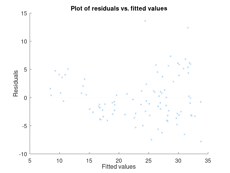
Spotting influential observations with Cook's distance. Sixteen houses are matched by size and age to a sale price, but one house was sold far above what its size and age would predict. After fitting the model, plotDiagnostics with the cookd option highlights that single observation as having outsized influence on the fit.
 Size  = [80; 95; 110; 120; 65; 140; 100; 130; 90; 150; 75; 105; ...
          115; 85; 135; 125];
 Age   = [5; 10; 3; 8; 20; 2; 15; 6; 12; 1; 18; 9; 4; 14; 7; 11];
 Price = [200; 230; 260; 280; 150; 320; 240; 300; 210; 340; 170; ...
          250; 270; 190; 500; 290];
 X = [Size, Age];
 y = Price;
 mdl = fitlm (X, y);
 plotDiagnostics (mdl, 'cookd')
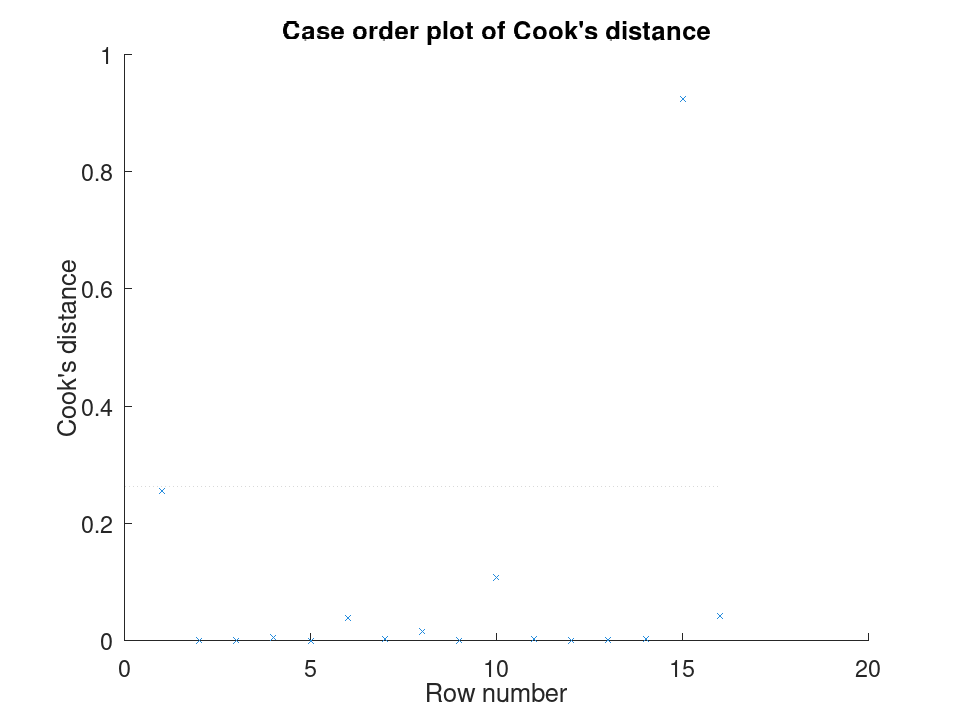
Comparing the size of each predictor's effect, alongside a hypothesis test on the model as a whole. We fit a mileage model on the carsmall data set using weight and horsepower. plotEffects draws each coefficient's estimate with its confidence interval side by side, and coefTest checks whether weight's effect is significantly different from horsepower's.
 load carsmall
 X = [Weight, Horsepower];
 y = MPG;
 mdl = fitlm (X, y);
Visualize the relative size of each predictor's effect.
plotEffects (mdl)
Test whether the two coefficients differ significantly.
 H = [0 1 -1];
 [p, F, r] = coefTest (mdl, H)
p = 0.073643
F = 3.2759
r = 1
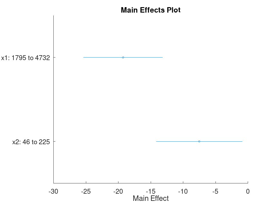
A scalar numeric value equal to SSE / DFE, where SSE is
the sum of squared errors and DFE is the degrees of freedom for
error. This property is read-only.
Simple linear regression with a single predictor. Ten runners record their weekly training distance and their finish time in a 10k race. We fit a straight line through this data and look at the fitted coefficients, then use predict to estimate the finish time for a runner who trains a distance not in the sample.
 Distance = [10; 15; 20; 25; 30; 35; 40; 45; 50; 55];
 Time     = [58; 55; 52; 50; 47; 45; 43; 41; 40; 38];
 X = Distance;
 y = Time;
Fit the model and inspect the estimated slope and intercept.
mdl = fitlm (X, y)
mdl =

  Linear regression model:
      y ~ 1 + x1

  Estimated Coefficients:

  2x4 table

                   Estimate       SE         tStat        pValue
                   ________    _________    ________    ___________

    (Intercept)        61.2     0.654588      93.494    1.91213e-13
    x1                -0.44    0.0184226    -23.8836    1.00609e-08


Number of observations: 10, Error degrees of freedom: 8
Root Mean Squared Error: 0.83666
R-squared: 0.986169,  Adjusted R-Squared: 0.984441
F-statistic vs. constant model: 570.429, p-value = 1.00609e-08
Predict the finish time for a runner training 32 km per week.
ypred = predict (mdl, 32)
ypred = 47.120
Multiple linear regression with two predictors, followed by a confidence interval on the coefficients. Thirteen coffee shops report their weekly foot traffic and the number of items on their menu, along with weekly revenue. We fit a model with both predictors, then use coefCI to see how precisely each coefficient is estimated.
 Traffic = [120; 150; 90; 200; 175; 60; 220; 140; 100; 190; 80; 210; 130];
 MenuSize = [8; 12; 6; 15; 10; 5; 18; 9; 7; 14; 6; 16; 11];
 Revenue = [1450; 1820; 1010; 2400; 2050; 700; 2650; 1700; 1150; ...
            2300; 900; 2500; 1600];
 X = [Traffic, MenuSize];
 y = Revenue;
Fit the model with both predictors together.
mdl = fitlm (X, y)
mdl =

  Linear regression model:
      y ~ 1 + x1 + x2

  Estimated Coefficients:

  3x4 table

                   Estimate       SE        tStat        pValue
                   ________    ________    ________    ___________

    (Intercept)    -47.0932     27.3456    -1.72215       0.115771
    x1              11.4079    0.616078      18.517    4.55169e-09
    x2              11.4344     7.68384     1.48811       0.167562


Number of observations: 13, Error degrees of freedom: 10
Root Mean Squared Error: 32.4551
R-squared: 0.997901,  Adjusted R-Squared: 0.997482
F-statistic vs. constant model: 2377.53, p-value = 4.07061e-14
Check how tight the 95% confidence interval is on each coefficient.
ci = coefCI (mdl)
ci =

  -108.0231    13.8366
    10.0352    12.7806
    -5.6862    28.5551
Growing a model with addTerms and predicting with the richer model. We model fuel economy from the carsmall data set using weight and horsepower as main effects only. addTerms then brings in the weight-horsepower interaction without needing to refit by hand, and predict shows how the estimate for a new car changes once that interaction is included.
 load carsmall
 X = [Weight, Horsepower];
 y = MPG;
Fit the additive model first.
mdl = fitlm (X, y);
Add the interaction between weight and horsepower.
mdl2 = addTerms (mdl, 'x1:x2');
Compare predictions from both models for the same new car.
 Xnew = [3200, 120];
 ypred1 = predict (mdl, Xnew)
ypred1 = 21.719
ypred2 = predict (mdl2, Xnew)
ypred2 = 20.416
Simplifying a model with removeTerms and comparing fit quality. We fit the full Hald cement model with all four ingredients, then use removeTerms to drop the weakest predictor and refit automatically. Comparing SSE before and after shows how little explanatory power that ingredient was actually contributing.
 load hald
 X = ingredients;
 y = heat;
Fit the model with all four ingredients.
mdl = fitlm (X, y);
Drop the third ingredient and refit on the same data.
mdl2 = removeTerms (mdl, 'x3');
Compare how much the error sum of squares changed.
sse_full = mdl.SSE
sse_full = 47.864
sse_reduced = mdl2.SSE
sse_reduced = 47.973
Testing a linear hypothesis and checking residual autocorrelation. Twelve patients are given a drug at different doses over different treatment durations, and a recovery score is recorded. coefTest checks whether the dose and duration coefficients are actually equal, and dwtest separately checks whether the residuals still carry a leftover pattern the model failed to capture.
 Dose     = [10; 15; 20; 25; 30; 35; 12; 18; 22; 28; 32; 38];
 Duration = [5; 7; 9; 11; 13; 15; 6; 8; 10; 12; 14; 16];
 Recovery = [42; 48; 55; 60; 68; 74; 45; 52; 58; 65; 71; 78];
 X = [Dose, Duration];
 y = Recovery;
 mdl = fitlm (X, y);
Test H0: the Dose and Duration coefficients are equal.
 H = [0 1 -1];
 [p, F, r] = coefTest (mdl, H)
p = 0.3535
F = 0.9571
r = 1
Check for autocorrelation left over in the residuals.
[pdw, dw] = dwtest (mdl)
pdw = 0.3658
dw = 2.4432
Checking residuals against fitted values. We fit a mileage model on the carsmall data set using weight and horsepower, then plot the raw residuals against the fitted values. A pattern in this plot, rather than a random scatter, would suggest the linear model is missing some curvature in the relationship.
load carsmall X = [Weight, Horsepower]; y = MPG; mdl = fitlm (X, y); plotResiduals (mdl, 'fitted')
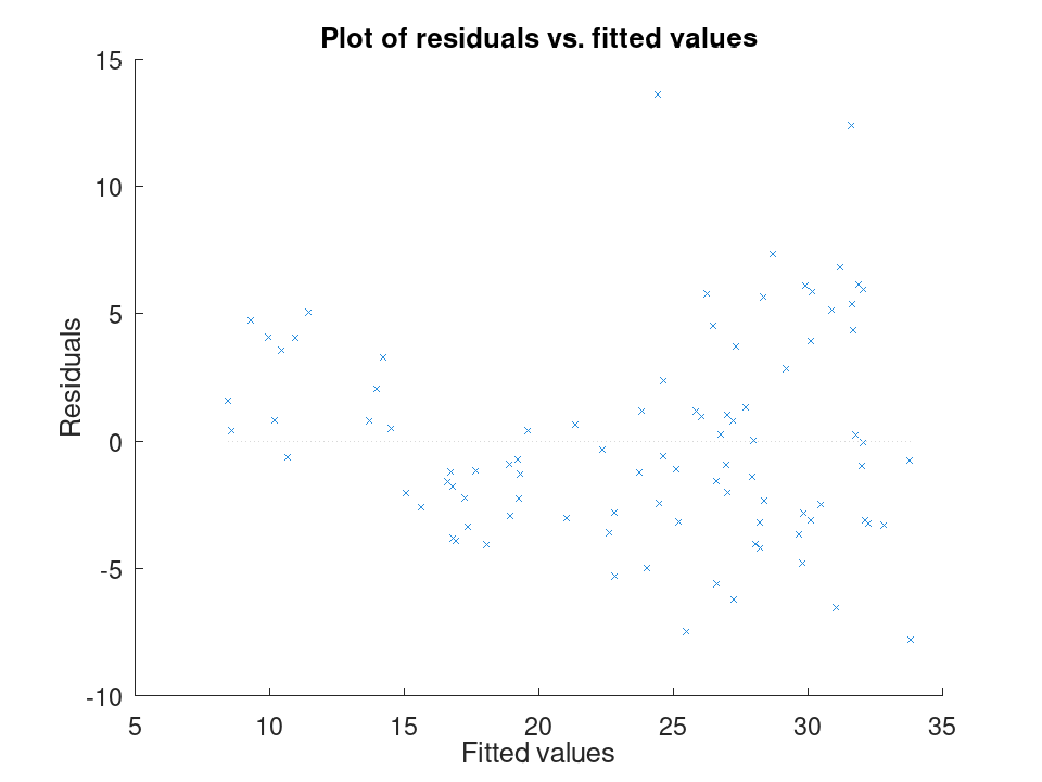
Spotting influential observations with Cook's distance. Sixteen houses are matched by size and age to a sale price, but one house was sold far above what its size and age would predict. After fitting the model, plotDiagnostics with the cookd option highlights that single observation as having outsized influence on the fit.
Size = [80; 95; 110; 120; 65; 140; 100; 130; 90; 150; 75; 105; ...
115; 85; 135; 125];
Age = [5; 10; 3; 8; 20; 2; 15; 6; 12; 1; 18; 9; 4; 14; 7; 11];
Price = [200; 230; 260; 280; 150; 320; 240; 300; 210; 340; 170; ...
250; 270; 190; 500; 290];
X = [Size, Age];
y = Price;
mdl = fitlm (X, y);
plotDiagnostics (mdl, 'cookd')
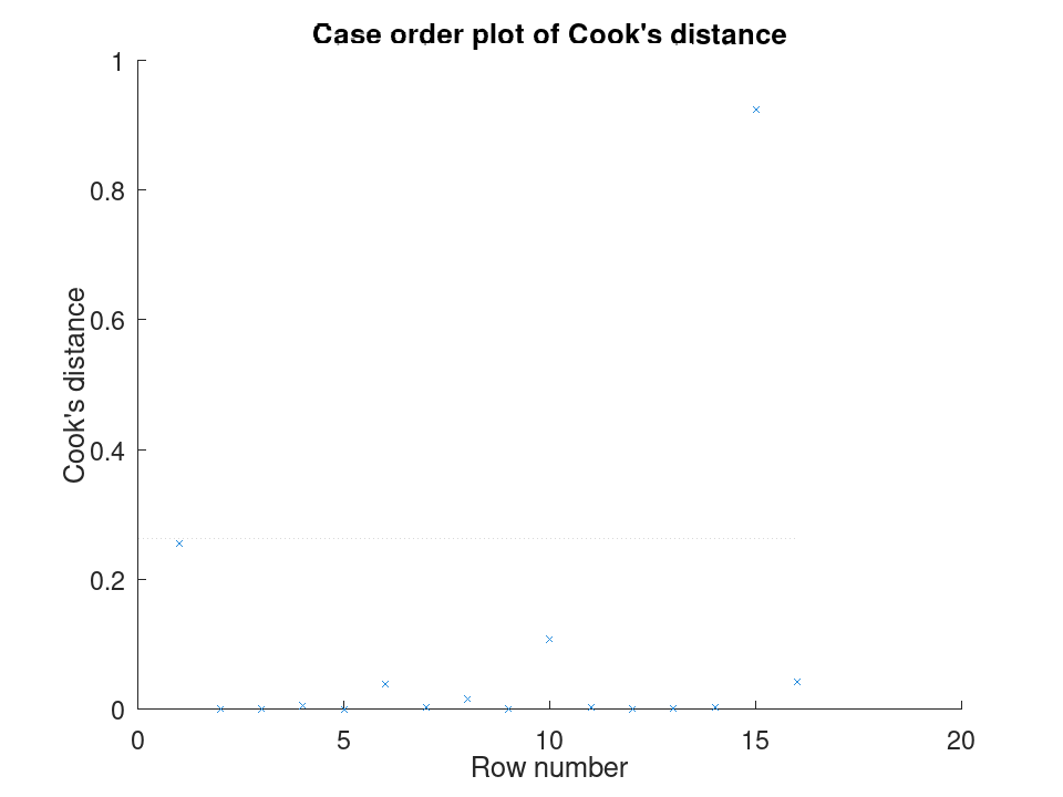
Comparing the size of each predictor's effect, alongside a hypothesis test on the model as a whole. We fit a mileage model on the carsmall data set using weight and horsepower. plotEffects draws each coefficient's estimate with its confidence interval side by side, and coefTest checks whether weight's effect is significantly different from horsepower's.
load carsmall X = [Weight, Horsepower]; y = MPG; mdl = fitlm (X, y);
Visualize the relative size of each predictor's effect.
plotEffects (mdl)
Test whether the two coefficients differ significantly.
H = [0 1 -1]; [p, F, r] = coefTest (mdl, H)
p = 0.073643 F = 3.2759 r = 1
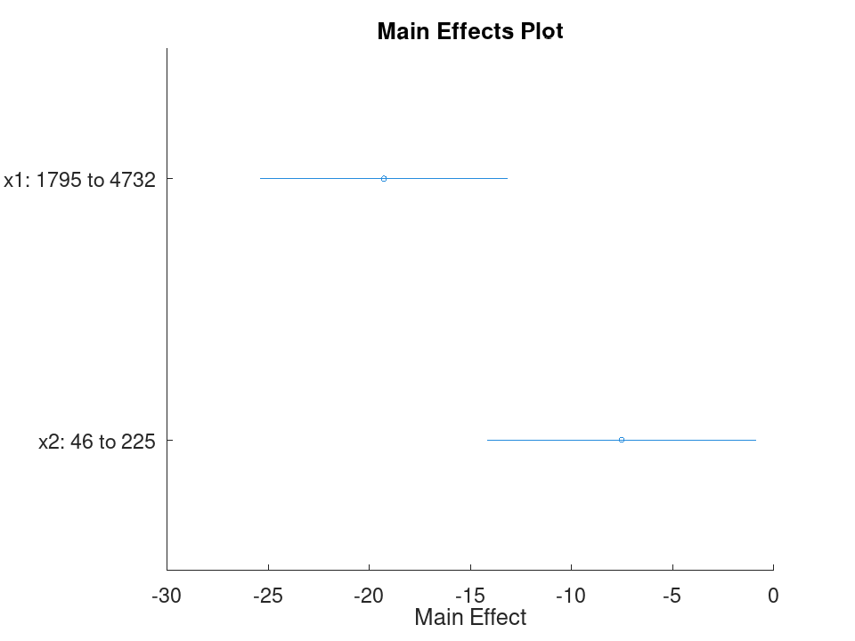
A table with one row per observation and four columns:
-
Raw- observed minus fitted values -
Pearson- raw residuals divided byRMSE -
Standardized- internally studentized residuals; raw residuals divided by their estimated standard deviation using the full-modelMSE -
Studentized- externally studentized residuals; each raw residual divided by an estimate of the standard deviation based on all observations except that one, using the delete-1S2_i
Rows not used in the fit contain NaN. This property is
read-only.
Simple linear regression with a single predictor. Ten runners record their weekly training distance and their finish time in a 10k race. We fit a straight line through this data and look at the fitted coefficients, then use predict to estimate the finish time for a runner who trains a distance not in the sample.
Distance = [10; 15; 20; 25; 30; 35; 40; 45; 50; 55]; Time = [58; 55; 52; 50; 47; 45; 43; 41; 40; 38]; X = Distance; y = Time;
Fit the model and inspect the estimated slope and intercept.
mdl = fitlm (X, y)
mdl =
Linear regression model:
y ~ 1 + x1
Estimated Coefficients:
2x4 table
Estimate SE tStat pValue
________ _________ ________ ___________
(Intercept) 61.2 0.654588 93.494 1.91213e-13
x1 -0.44 0.0184226 -23.8836 1.00609e-08
Number of observations: 10, Error degrees of freedom: 8
Root Mean Squared Error: 0.83666
R-squared: 0.986169, Adjusted R-Squared: 0.984441
F-statistic vs. constant model: 570.429, p-value = 1.00609e-08
Predict the finish time for a runner training 32 km per week.
ypred = predict (mdl, 32)
ypred = 47.120
Multiple linear regression with two predictors, followed by a confidence interval on the coefficients. Thirteen coffee shops report their weekly foot traffic and the number of items on their menu, along with weekly revenue. We fit a model with both predictors, then use coefCI to see how precisely each coefficient is estimated.
Traffic = [120; 150; 90; 200; 175; 60; 220; 140; 100; 190; 80; 210; 130];
MenuSize = [8; 12; 6; 15; 10; 5; 18; 9; 7; 14; 6; 16; 11];
Revenue = [1450; 1820; 1010; 2400; 2050; 700; 2650; 1700; 1150; ...
2300; 900; 2500; 1600];
X = [Traffic, MenuSize];
y = Revenue;
Fit the model with both predictors together.
mdl = fitlm (X, y)
mdl =
Linear regression model:
y ~ 1 + x1 + x2
Estimated Coefficients:
3x4 table
Estimate SE tStat pValue
________ ________ ________ ___________
(Intercept) -47.0932 27.3456 -1.72215 0.115771
x1 11.4079 0.616078 18.517 4.55169e-09
x2 11.4344 7.68384 1.48811 0.167562
Number of observations: 13, Error degrees of freedom: 10
Root Mean Squared Error: 32.4551
R-squared: 0.997901, Adjusted R-Squared: 0.997482
F-statistic vs. constant model: 2377.53, p-value = 4.07061e-14
Check how tight the 95% confidence interval is on each coefficient.
ci = coefCI (mdl)
ci =
-108.0231 13.8366
10.0352 12.7806
-5.6862 28.5551
Growing a model with addTerms and predicting with the richer model. We model fuel economy from the carsmall data set using weight and horsepower as main effects only. addTerms then brings in the weight-horsepower interaction without needing to refit by hand, and predict shows how the estimate for a new car changes once that interaction is included.
load carsmall X = [Weight, Horsepower]; y = MPG;
Fit the additive model first.
mdl = fitlm (X, y);
Add the interaction between weight and horsepower.
mdl2 = addTerms (mdl, 'x1:x2');
Compare predictions from both models for the same new car.
Xnew = [3200, 120]; ypred1 = predict (mdl, Xnew)
ypred1 = 21.719
ypred2 = predict (mdl2, Xnew)
ypred2 = 20.416
Simplifying a model with removeTerms and comparing fit quality. We fit the full Hald cement model with all four ingredients, then use removeTerms to drop the weakest predictor and refit automatically. Comparing SSE before and after shows how little explanatory power that ingredient was actually contributing.
load hald X = ingredients; y = heat;
Fit the model with all four ingredients.
mdl = fitlm (X, y);
Drop the third ingredient and refit on the same data.
mdl2 = removeTerms (mdl, 'x3');
Compare how much the error sum of squares changed.
sse_full = mdl.SSE
sse_full = 47.864
sse_reduced = mdl2.SSE
sse_reduced = 47.973
Testing a linear hypothesis and checking residual autocorrelation. Twelve patients are given a drug at different doses over different treatment durations, and a recovery score is recorded. coefTest checks whether the dose and duration coefficients are actually equal, and dwtest separately checks whether the residuals still carry a leftover pattern the model failed to capture.
Dose = [10; 15; 20; 25; 30; 35; 12; 18; 22; 28; 32; 38]; Duration = [5; 7; 9; 11; 13; 15; 6; 8; 10; 12; 14; 16]; Recovery = [42; 48; 55; 60; 68; 74; 45; 52; 58; 65; 71; 78]; X = [Dose, Duration]; y = Recovery; mdl = fitlm (X, y);
Test H0: the Dose and Duration coefficients are equal.
H = [0 1 -1]; [p, F, r] = coefTest (mdl, H)
p = 0.3535 F = 0.9571 r = 1
Check for autocorrelation left over in the residuals.
[pdw, dw] = dwtest (mdl)
pdw = 0.3658 dw = 2.4432
Checking residuals against fitted values. We fit a mileage model on the carsmall data set using weight and horsepower, then plot the raw residuals against the fitted values. A pattern in this plot, rather than a random scatter, would suggest the linear model is missing some curvature in the relationship.
load carsmall X = [Weight, Horsepower]; y = MPG; mdl = fitlm (X, y); plotResiduals (mdl, 'fitted')
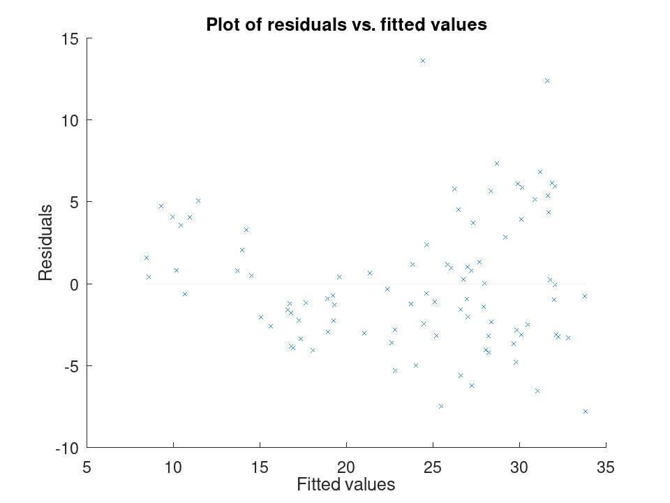
Spotting influential observations with Cook's distance. Sixteen houses are matched by size and age to a sale price, but one house was sold far above what its size and age would predict. After fitting the model, plotDiagnostics with the cookd option highlights that single observation as having outsized influence on the fit.
Size = [80; 95; 110; 120; 65; 140; 100; 130; 90; 150; 75; 105; ...
115; 85; 135; 125];
Age = [5; 10; 3; 8; 20; 2; 15; 6; 12; 1; 18; 9; 4; 14; 7; 11];
Price = [200; 230; 260; 280; 150; 320; 240; 300; 210; 340; 170; ...
250; 270; 190; 500; 290];
X = [Size, Age];
y = Price;
mdl = fitlm (X, y);
plotDiagnostics (mdl, 'cookd')
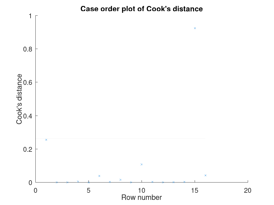
Comparing the size of each predictor's effect, alongside a hypothesis test on the model as a whole. We fit a mileage model on the carsmall data set using weight and horsepower. plotEffects draws each coefficient's estimate with its confidence interval side by side, and coefTest checks whether weight's effect is significantly different from horsepower's.
load carsmall X = [Weight, Horsepower]; y = MPG; mdl = fitlm (X, y);
Visualize the relative size of each predictor's effect.
plotEffects (mdl)
Test whether the two coefficients differ significantly.
H = [0 1 -1]; [p, F, r] = coefTest (mdl, H)
p = 0.073643 F = 3.2759 r = 1
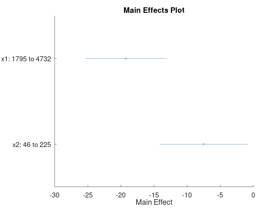
A scalar numeric value equal to sqrt(MSE). This property is read-only.
Simple linear regression with a single predictor. Ten runners record their weekly training distance and their finish time in a 10k race. We fit a straight line through this data and look at the fitted coefficients, then use predict to estimate the finish time for a runner who trains a distance not in the sample.
Distance = [10; 15; 20; 25; 30; 35; 40; 45; 50; 55]; Time = [58; 55; 52; 50; 47; 45; 43; 41; 40; 38]; X = Distance; y = Time;
Fit the model and inspect the estimated slope and intercept.
mdl = fitlm (X, y)
mdl =
Linear regression model:
y ~ 1 + x1
Estimated Coefficients:
2x4 table
Estimate SE tStat pValue
________ _________ ________ ___________
(Intercept) 61.2 0.654588 93.494 1.91213e-13
x1 -0.44 0.0184226 -23.8836 1.00609e-08
Number of observations: 10, Error degrees of freedom: 8
Root Mean Squared Error: 0.83666
R-squared: 0.986169, Adjusted R-Squared: 0.984441
F-statistic vs. constant model: 570.429, p-value = 1.00609e-08
Predict the finish time for a runner training 32 km per week.
ypred = predict (mdl, 32)
ypred = 47.120
Multiple linear regression with two predictors, followed by a confidence interval on the coefficients. Thirteen coffee shops report their weekly foot traffic and the number of items on their menu, along with weekly revenue. We fit a model with both predictors, then use coefCI to see how precisely each coefficient is estimated.
Traffic = [120; 150; 90; 200; 175; 60; 220; 140; 100; 190; 80; 210; 130];
MenuSize = [8; 12; 6; 15; 10; 5; 18; 9; 7; 14; 6; 16; 11];
Revenue = [1450; 1820; 1010; 2400; 2050; 700; 2650; 1700; 1150; ...
2300; 900; 2500; 1600];
X = [Traffic, MenuSize];
y = Revenue;
Fit the model with both predictors together.
mdl = fitlm (X, y)
mdl =
Linear regression model:
y ~ 1 + x1 + x2
Estimated Coefficients:
3x4 table
Estimate SE tStat pValue
________ ________ ________ ___________
(Intercept) -47.0932 27.3456 -1.72215 0.115771
x1 11.4079 0.616078 18.517 4.55169e-09
x2 11.4344 7.68384 1.48811 0.167562
Number of observations: 13, Error degrees of freedom: 10
Root Mean Squared Error: 32.4551
R-squared: 0.997901, Adjusted R-Squared: 0.997482
F-statistic vs. constant model: 2377.53, p-value = 4.07061e-14
Check how tight the 95% confidence interval is on each coefficient.
ci = coefCI (mdl)
ci =
-108.0231 13.8366
10.0352 12.7806
-5.6862 28.5551
Growing a model with addTerms and predicting with the richer model. We model fuel economy from the carsmall data set using weight and horsepower as main effects only. addTerms then brings in the weight-horsepower interaction without needing to refit by hand, and predict shows how the estimate for a new car changes once that interaction is included.
load carsmall X = [Weight, Horsepower]; y = MPG;
Fit the additive model first.
mdl = fitlm (X, y);
Add the interaction between weight and horsepower.
mdl2 = addTerms (mdl, 'x1:x2');
Compare predictions from both models for the same new car.
Xnew = [3200, 120]; ypred1 = predict (mdl, Xnew)
ypred1 = 21.719
ypred2 = predict (mdl2, Xnew)
ypred2 = 20.416
Simplifying a model with removeTerms and comparing fit quality. We fit the full Hald cement model with all four ingredients, then use removeTerms to drop the weakest predictor and refit automatically. Comparing SSE before and after shows how little explanatory power that ingredient was actually contributing.
load hald X = ingredients; y = heat;
Fit the model with all four ingredients.
mdl = fitlm (X, y);
Drop the third ingredient and refit on the same data.
mdl2 = removeTerms (mdl, 'x3');
Compare how much the error sum of squares changed.
sse_full = mdl.SSE
sse_full = 47.864
sse_reduced = mdl2.SSE
sse_reduced = 47.973
Testing a linear hypothesis and checking residual autocorrelation. Twelve patients are given a drug at different doses over different treatment durations, and a recovery score is recorded. coefTest checks whether the dose and duration coefficients are actually equal, and dwtest separately checks whether the residuals still carry a leftover pattern the model failed to capture.
Dose = [10; 15; 20; 25; 30; 35; 12; 18; 22; 28; 32; 38]; Duration = [5; 7; 9; 11; 13; 15; 6; 8; 10; 12; 14; 16]; Recovery = [42; 48; 55; 60; 68; 74; 45; 52; 58; 65; 71; 78]; X = [Dose, Duration]; y = Recovery; mdl = fitlm (X, y);
Test H0: the Dose and Duration coefficients are equal.
H = [0 1 -1]; [p, F, r] = coefTest (mdl, H)
p = 0.3535 F = 0.9571 r = 1
Check for autocorrelation left over in the residuals.
[pdw, dw] = dwtest (mdl)
pdw = 0.3658 dw = 2.4432
Checking residuals against fitted values. We fit a mileage model on the carsmall data set using weight and horsepower, then plot the raw residuals against the fitted values. A pattern in this plot, rather than a random scatter, would suggest the linear model is missing some curvature in the relationship.
load carsmall X = [Weight, Horsepower]; y = MPG; mdl = fitlm (X, y); plotResiduals (mdl, 'fitted')
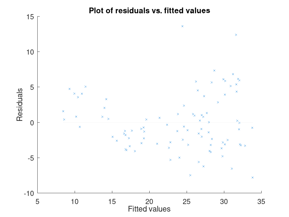
Spotting influential observations with Cook's distance. Sixteen houses are matched by size and age to a sale price, but one house was sold far above what its size and age would predict. After fitting the model, plotDiagnostics with the cookd option highlights that single observation as having outsized influence on the fit.
Size = [80; 95; 110; 120; 65; 140; 100; 130; 90; 150; 75; 105; ...
115; 85; 135; 125];
Age = [5; 10; 3; 8; 20; 2; 15; 6; 12; 1; 18; 9; 4; 14; 7; 11];
Price = [200; 230; 260; 280; 150; 320; 240; 300; 210; 340; 170; ...
250; 270; 190; 500; 290];
X = [Size, Age];
y = Price;
mdl = fitlm (X, y);
plotDiagnostics (mdl, 'cookd')
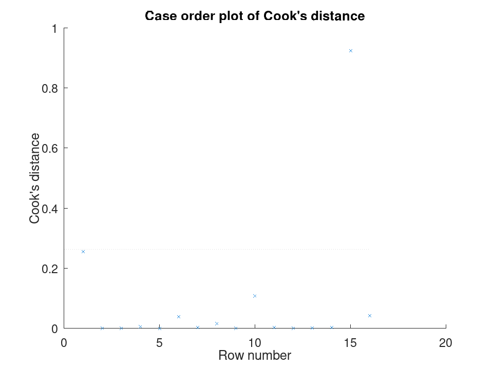
Comparing the size of each predictor's effect, alongside a hypothesis test on the model as a whole. We fit a mileage model on the carsmall data set using weight and horsepower. plotEffects draws each coefficient's estimate with its confidence interval side by side, and coefTest checks whether weight's effect is significantly different from horsepower's.
load carsmall X = [Weight, Horsepower]; y = MPG; mdl = fitlm (X, y);
Visualize the relative size of each predictor's effect.
plotEffects (mdl)
Test whether the two coefficients differ significantly.
H = [0 1 -1]; [p, F, r] = coefTest (mdl, H)
p = 0.073643 F = 3.2759 r = 1
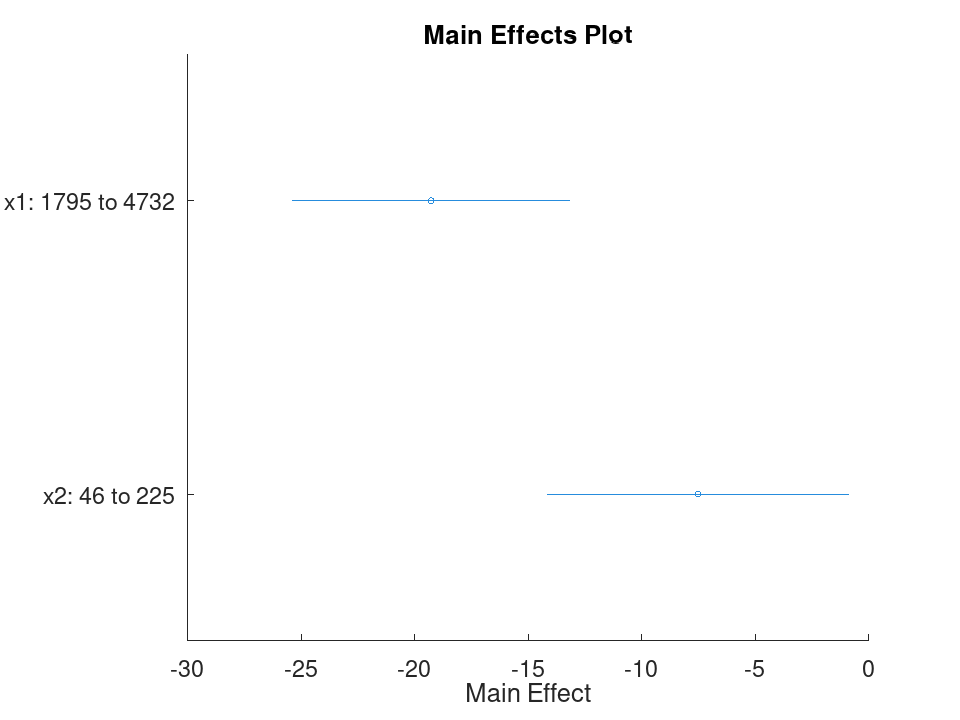
A structure with two fields:
-
Ordinary- coefficient of determination: R^2 = SSR / SST -
Adjusted- adjusted R^2 that accounts for the number of coefficients in the model
This property is read-only.
Simple linear regression with a single predictor. Ten runners record their weekly training distance and their finish time in a 10k race. We fit a straight line through this data and look at the fitted coefficients, then use predict to estimate the finish time for a runner who trains a distance not in the sample.
Distance = [10; 15; 20; 25; 30; 35; 40; 45; 50; 55]; Time = [58; 55; 52; 50; 47; 45; 43; 41; 40; 38]; X = Distance; y = Time;
Fit the model and inspect the estimated slope and intercept.
mdl = fitlm (X, y)
mdl =
Linear regression model:
y ~ 1 + x1
Estimated Coefficients:
2x4 table
Estimate SE tStat pValue
________ _________ ________ ___________
(Intercept) 61.2 0.654588 93.494 1.91213e-13
x1 -0.44 0.0184226 -23.8836 1.00609e-08
Number of observations: 10, Error degrees of freedom: 8
Root Mean Squared Error: 0.83666
R-squared: 0.986169, Adjusted R-Squared: 0.984441
F-statistic vs. constant model: 570.429, p-value = 1.00609e-08
Predict the finish time for a runner training 32 km per week.
ypred = predict (mdl, 32)
ypred = 47.120
Multiple linear regression with two predictors, followed by a confidence interval on the coefficients. Thirteen coffee shops report their weekly foot traffic and the number of items on their menu, along with weekly revenue. We fit a model with both predictors, then use coefCI to see how precisely each coefficient is estimated.
Traffic = [120; 150; 90; 200; 175; 60; 220; 140; 100; 190; 80; 210; 130];
MenuSize = [8; 12; 6; 15; 10; 5; 18; 9; 7; 14; 6; 16; 11];
Revenue = [1450; 1820; 1010; 2400; 2050; 700; 2650; 1700; 1150; ...
2300; 900; 2500; 1600];
X = [Traffic, MenuSize];
y = Revenue;
Fit the model with both predictors together.
mdl = fitlm (X, y)
mdl =
Linear regression model:
y ~ 1 + x1 + x2
Estimated Coefficients:
3x4 table
Estimate SE tStat pValue
________ ________ ________ ___________
(Intercept) -47.0932 27.3456 -1.72215 0.115771
x1 11.4079 0.616078 18.517 4.55169e-09
x2 11.4344 7.68384 1.48811 0.167562
Number of observations: 13, Error degrees of freedom: 10
Root Mean Squared Error: 32.4551
R-squared: 0.997901, Adjusted R-Squared: 0.997482
F-statistic vs. constant model: 2377.53, p-value = 4.07061e-14
Check how tight the 95% confidence interval is on each coefficient.
ci = coefCI (mdl)
ci =
-108.0231 13.8366
10.0352 12.7806
-5.6862 28.5551
Growing a model with addTerms and predicting with the richer model. We model fuel economy from the carsmall data set using weight and horsepower as main effects only. addTerms then brings in the weight-horsepower interaction without needing to refit by hand, and predict shows how the estimate for a new car changes once that interaction is included.
load carsmall X = [Weight, Horsepower]; y = MPG;
Fit the additive model first.
mdl = fitlm (X, y);
Add the interaction between weight and horsepower.
mdl2 = addTerms (mdl, 'x1:x2');
Compare predictions from both models for the same new car.
Xnew = [3200, 120]; ypred1 = predict (mdl, Xnew)
ypred1 = 21.719
ypred2 = predict (mdl2, Xnew)
ypred2 = 20.416
Simplifying a model with removeTerms and comparing fit quality. We fit the full Hald cement model with all four ingredients, then use removeTerms to drop the weakest predictor and refit automatically. Comparing SSE before and after shows how little explanatory power that ingredient was actually contributing.
load hald X = ingredients; y = heat;
Fit the model with all four ingredients.
mdl = fitlm (X, y);
Drop the third ingredient and refit on the same data.
mdl2 = removeTerms (mdl, 'x3');
Compare how much the error sum of squares changed.
sse_full = mdl.SSE
sse_full = 47.864
sse_reduced = mdl2.SSE
sse_reduced = 47.973
Testing a linear hypothesis and checking residual autocorrelation. Twelve patients are given a drug at different doses over different treatment durations, and a recovery score is recorded. coefTest checks whether the dose and duration coefficients are actually equal, and dwtest separately checks whether the residuals still carry a leftover pattern the model failed to capture.
Dose = [10; 15; 20; 25; 30; 35; 12; 18; 22; 28; 32; 38]; Duration = [5; 7; 9; 11; 13; 15; 6; 8; 10; 12; 14; 16]; Recovery = [42; 48; 55; 60; 68; 74; 45; 52; 58; 65; 71; 78]; X = [Dose, Duration]; y = Recovery; mdl = fitlm (X, y);
Test H0: the Dose and Duration coefficients are equal.
H = [0 1 -1]; [p, F, r] = coefTest (mdl, H)
p = 0.3535 F = 0.9571 r = 1
Check for autocorrelation left over in the residuals.
[pdw, dw] = dwtest (mdl)
pdw = 0.3658 dw = 2.4432
Checking residuals against fitted values. We fit a mileage model on the carsmall data set using weight and horsepower, then plot the raw residuals against the fitted values. A pattern in this plot, rather than a random scatter, would suggest the linear model is missing some curvature in the relationship.
load carsmall X = [Weight, Horsepower]; y = MPG; mdl = fitlm (X, y); plotResiduals (mdl, 'fitted')
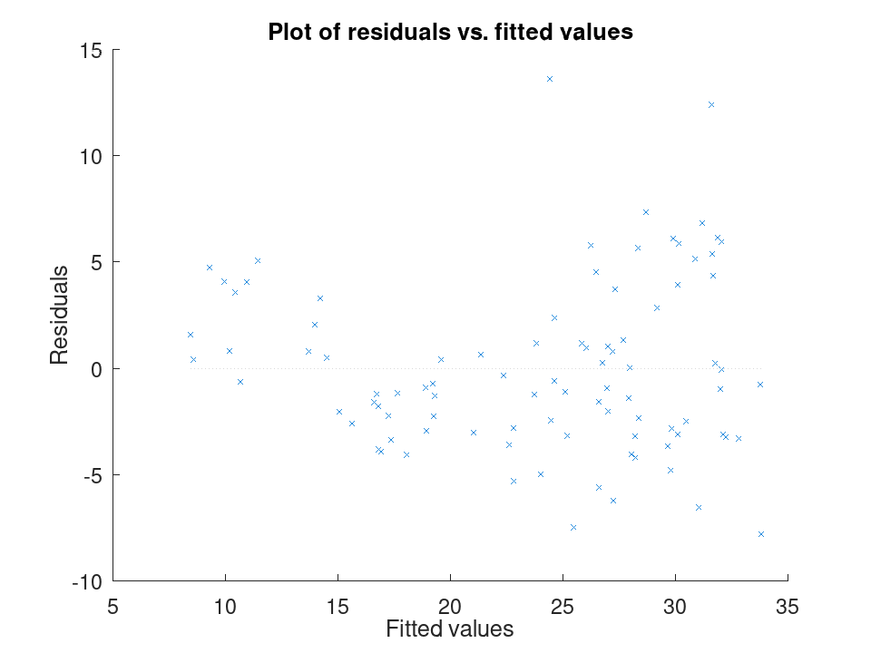
Spotting influential observations with Cook's distance. Sixteen houses are matched by size and age to a sale price, but one house was sold far above what its size and age would predict. After fitting the model, plotDiagnostics with the cookd option highlights that single observation as having outsized influence on the fit.
Size = [80; 95; 110; 120; 65; 140; 100; 130; 90; 150; 75; 105; ...
115; 85; 135; 125];
Age = [5; 10; 3; 8; 20; 2; 15; 6; 12; 1; 18; 9; 4; 14; 7; 11];
Price = [200; 230; 260; 280; 150; 320; 240; 300; 210; 340; 170; ...
250; 270; 190; 500; 290];
X = [Size, Age];
y = Price;
mdl = fitlm (X, y);
plotDiagnostics (mdl, 'cookd')
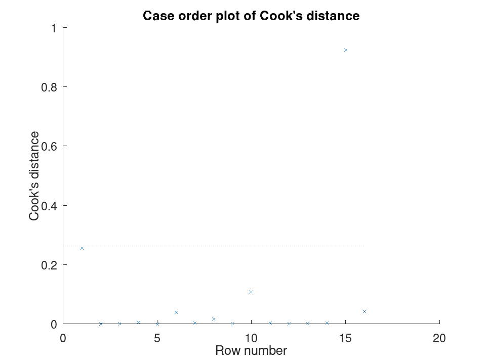
Comparing the size of each predictor's effect, alongside a hypothesis test on the model as a whole. We fit a mileage model on the carsmall data set using weight and horsepower. plotEffects draws each coefficient's estimate with its confidence interval side by side, and coefTest checks whether weight's effect is significantly different from horsepower's.
load carsmall X = [Weight, Horsepower]; y = MPG; mdl = fitlm (X, y);
Visualize the relative size of each predictor's effect.
plotEffects (mdl)
Test whether the two coefficients differ significantly.
H = [0 1 -1]; [p, F, r] = coefTest (mdl, H)
p = 0.073643 F = 3.2759 r = 1
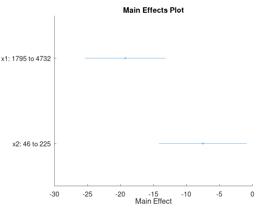
A scalar numeric value equal to the sum of squared residuals. For a model with an intercept, SST = SSE + SSR. For weighted fits, this is the weighted sum of squares. This property is read-only.
Simple linear regression with a single predictor. Ten runners record their weekly training distance and their finish time in a 10k race. We fit a straight line through this data and look at the fitted coefficients, then use predict to estimate the finish time for a runner who trains a distance not in the sample.
Distance = [10; 15; 20; 25; 30; 35; 40; 45; 50; 55]; Time = [58; 55; 52; 50; 47; 45; 43; 41; 40; 38]; X = Distance; y = Time;
Fit the model and inspect the estimated slope and intercept.
mdl = fitlm (X, y)
mdl =
Linear regression model:
y ~ 1 + x1
Estimated Coefficients:
2x4 table
Estimate SE tStat pValue
________ _________ ________ ___________
(Intercept) 61.2 0.654588 93.494 1.91213e-13
x1 -0.44 0.0184226 -23.8836 1.00609e-08
Number of observations: 10, Error degrees of freedom: 8
Root Mean Squared Error: 0.83666
R-squared: 0.986169, Adjusted R-Squared: 0.984441
F-statistic vs. constant model: 570.429, p-value = 1.00609e-08
Predict the finish time for a runner training 32 km per week.
ypred = predict (mdl, 32)
ypred = 47.120
Multiple linear regression with two predictors, followed by a confidence interval on the coefficients. Thirteen coffee shops report their weekly foot traffic and the number of items on their menu, along with weekly revenue. We fit a model with both predictors, then use coefCI to see how precisely each coefficient is estimated.
Traffic = [120; 150; 90; 200; 175; 60; 220; 140; 100; 190; 80; 210; 130];
MenuSize = [8; 12; 6; 15; 10; 5; 18; 9; 7; 14; 6; 16; 11];
Revenue = [1450; 1820; 1010; 2400; 2050; 700; 2650; 1700; 1150; ...
2300; 900; 2500; 1600];
X = [Traffic, MenuSize];
y = Revenue;
Fit the model with both predictors together.
mdl = fitlm (X, y)
mdl =
Linear regression model:
y ~ 1 + x1 + x2
Estimated Coefficients:
3x4 table
Estimate SE tStat pValue
________ ________ ________ ___________
(Intercept) -47.0932 27.3456 -1.72215 0.115771
x1 11.4079 0.616078 18.517 4.55169e-09
x2 11.4344 7.68384 1.48811 0.167562
Number of observations: 13, Error degrees of freedom: 10
Root Mean Squared Error: 32.4551
R-squared: 0.997901, Adjusted R-Squared: 0.997482
F-statistic vs. constant model: 2377.53, p-value = 4.07061e-14
Check how tight the 95% confidence interval is on each coefficient.
ci = coefCI (mdl)
ci =
-108.0231 13.8366
10.0352 12.7806
-5.6862 28.5551
Growing a model with addTerms and predicting with the richer model. We model fuel economy from the carsmall data set using weight and horsepower as main effects only. addTerms then brings in the weight-horsepower interaction without needing to refit by hand, and predict shows how the estimate for a new car changes once that interaction is included.
load carsmall X = [Weight, Horsepower]; y = MPG;
Fit the additive model first.
mdl = fitlm (X, y);
Add the interaction between weight and horsepower.
mdl2 = addTerms (mdl, 'x1:x2');
Compare predictions from both models for the same new car.
Xnew = [3200, 120]; ypred1 = predict (mdl, Xnew)
ypred1 = 21.719
ypred2 = predict (mdl2, Xnew)
ypred2 = 20.416
Simplifying a model with removeTerms and comparing fit quality. We fit the full Hald cement model with all four ingredients, then use removeTerms to drop the weakest predictor and refit automatically. Comparing SSE before and after shows how little explanatory power that ingredient was actually contributing.
load hald X = ingredients; y = heat;
Fit the model with all four ingredients.
mdl = fitlm (X, y);
Drop the third ingredient and refit on the same data.
mdl2 = removeTerms (mdl, 'x3');
Compare how much the error sum of squares changed.
sse_full = mdl.SSE
sse_full = 47.864
sse_reduced = mdl2.SSE
sse_reduced = 47.973
Testing a linear hypothesis and checking residual autocorrelation. Twelve patients are given a drug at different doses over different treatment durations, and a recovery score is recorded. coefTest checks whether the dose and duration coefficients are actually equal, and dwtest separately checks whether the residuals still carry a leftover pattern the model failed to capture.
Dose = [10; 15; 20; 25; 30; 35; 12; 18; 22; 28; 32; 38]; Duration = [5; 7; 9; 11; 13; 15; 6; 8; 10; 12; 14; 16]; Recovery = [42; 48; 55; 60; 68; 74; 45; 52; 58; 65; 71; 78]; X = [Dose, Duration]; y = Recovery; mdl = fitlm (X, y);
Test H0: the Dose and Duration coefficients are equal.
H = [0 1 -1]; [p, F, r] = coefTest (mdl, H)
p = 0.3535 F = 0.9571 r = 1
Check for autocorrelation left over in the residuals.
[pdw, dw] = dwtest (mdl)
pdw = 0.3658 dw = 2.4432
Checking residuals against fitted values. We fit a mileage model on the carsmall data set using weight and horsepower, then plot the raw residuals against the fitted values. A pattern in this plot, rather than a random scatter, would suggest the linear model is missing some curvature in the relationship.
load carsmall X = [Weight, Horsepower]; y = MPG; mdl = fitlm (X, y); plotResiduals (mdl, 'fitted')
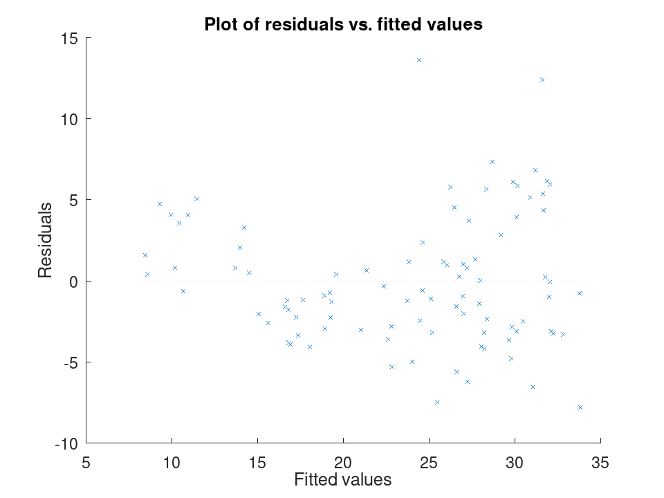
Spotting influential observations with Cook's distance. Sixteen houses are matched by size and age to a sale price, but one house was sold far above what its size and age would predict. After fitting the model, plotDiagnostics with the cookd option highlights that single observation as having outsized influence on the fit.
Size = [80; 95; 110; 120; 65; 140; 100; 130; 90; 150; 75; 105; ...
115; 85; 135; 125];
Age = [5; 10; 3; 8; 20; 2; 15; 6; 12; 1; 18; 9; 4; 14; 7; 11];
Price = [200; 230; 260; 280; 150; 320; 240; 300; 210; 340; 170; ...
250; 270; 190; 500; 290];
X = [Size, Age];
y = Price;
mdl = fitlm (X, y);
plotDiagnostics (mdl, 'cookd')
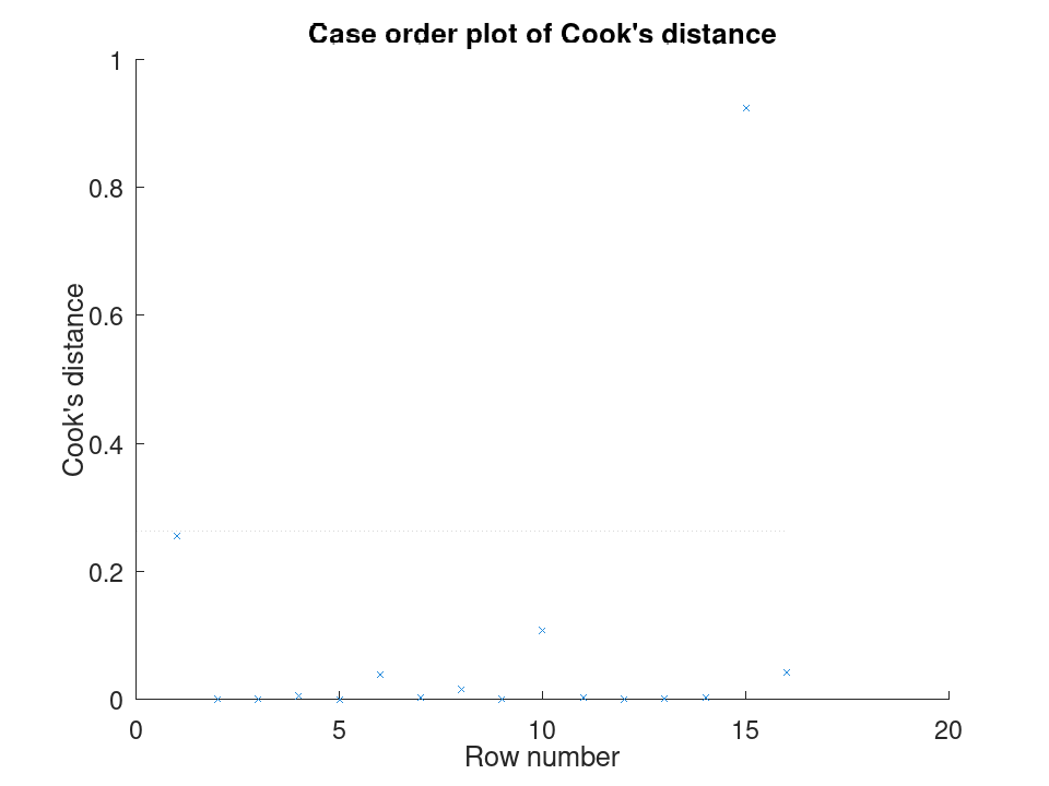
Comparing the size of each predictor's effect, alongside a hypothesis test on the model as a whole. We fit a mileage model on the carsmall data set using weight and horsepower. plotEffects draws each coefficient's estimate with its confidence interval side by side, and coefTest checks whether weight's effect is significantly different from horsepower's.
load carsmall X = [Weight, Horsepower]; y = MPG; mdl = fitlm (X, y);
Visualize the relative size of each predictor's effect.
plotEffects (mdl)
Test whether the two coefficients differ significantly.
H = [0 1 -1]; [p, F, r] = coefTest (mdl, H)
p = 0.073643 F = 3.2759 r = 1
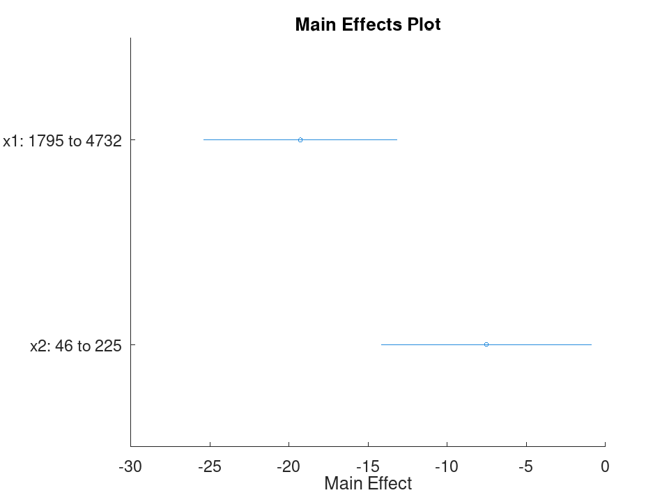
A scalar numeric value equal to the sum of squared deviations of the fitted values from the mean of the response. For a model with an intercept, SST = SSE + SSR. For weighted fits, this is the weighted sum of squares. This property is read-only.
Simple linear regression with a single predictor. Ten runners record their weekly training distance and their finish time in a 10k race. We fit a straight line through this data and look at the fitted coefficients, then use predict to estimate the finish time for a runner who trains a distance not in the sample.
Distance = [10; 15; 20; 25; 30; 35; 40; 45; 50; 55]; Time = [58; 55; 52; 50; 47; 45; 43; 41; 40; 38]; X = Distance; y = Time;
Fit the model and inspect the estimated slope and intercept.
mdl = fitlm (X, y)
mdl =
Linear regression model:
y ~ 1 + x1
Estimated Coefficients:
2x4 table
Estimate SE tStat pValue
________ _________ ________ ___________
(Intercept) 61.2 0.654588 93.494 1.91213e-13
x1 -0.44 0.0184226 -23.8836 1.00609e-08
Number of observations: 10, Error degrees of freedom: 8
Root Mean Squared Error: 0.83666
R-squared: 0.986169, Adjusted R-Squared: 0.984441
F-statistic vs. constant model: 570.429, p-value = 1.00609e-08
Predict the finish time for a runner training 32 km per week.
ypred = predict (mdl, 32)
ypred = 47.120
Multiple linear regression with two predictors, followed by a confidence interval on the coefficients. Thirteen coffee shops report their weekly foot traffic and the number of items on their menu, along with weekly revenue. We fit a model with both predictors, then use coefCI to see how precisely each coefficient is estimated.
Traffic = [120; 150; 90; 200; 175; 60; 220; 140; 100; 190; 80; 210; 130];
MenuSize = [8; 12; 6; 15; 10; 5; 18; 9; 7; 14; 6; 16; 11];
Revenue = [1450; 1820; 1010; 2400; 2050; 700; 2650; 1700; 1150; ...
2300; 900; 2500; 1600];
X = [Traffic, MenuSize];
y = Revenue;
Fit the model with both predictors together.
mdl = fitlm (X, y)
mdl =
Linear regression model:
y ~ 1 + x1 + x2
Estimated Coefficients:
3x4 table
Estimate SE tStat pValue
________ ________ ________ ___________
(Intercept) -47.0932 27.3456 -1.72215 0.115771
x1 11.4079 0.616078 18.517 4.55169e-09
x2 11.4344 7.68384 1.48811 0.167562
Number of observations: 13, Error degrees of freedom: 10
Root Mean Squared Error: 32.4551
R-squared: 0.997901, Adjusted R-Squared: 0.997482
F-statistic vs. constant model: 2377.53, p-value = 4.07061e-14
Check how tight the 95% confidence interval is on each coefficient.
ci = coefCI (mdl)
ci =
-108.0231 13.8366
10.0352 12.7806
-5.6862 28.5551
Growing a model with addTerms and predicting with the richer model. We model fuel economy from the carsmall data set using weight and horsepower as main effects only. addTerms then brings in the weight-horsepower interaction without needing to refit by hand, and predict shows how the estimate for a new car changes once that interaction is included.
load carsmall X = [Weight, Horsepower]; y = MPG;
Fit the additive model first.
mdl = fitlm (X, y);
Add the interaction between weight and horsepower.
mdl2 = addTerms (mdl, 'x1:x2');
Compare predictions from both models for the same new car.
Xnew = [3200, 120]; ypred1 = predict (mdl, Xnew)
ypred1 = 21.719
ypred2 = predict (mdl2, Xnew)
ypred2 = 20.416
Simplifying a model with removeTerms and comparing fit quality. We fit the full Hald cement model with all four ingredients, then use removeTerms to drop the weakest predictor and refit automatically. Comparing SSE before and after shows how little explanatory power that ingredient was actually contributing.
load hald X = ingredients; y = heat;
Fit the model with all four ingredients.
mdl = fitlm (X, y);
Drop the third ingredient and refit on the same data.
mdl2 = removeTerms (mdl, 'x3');
Compare how much the error sum of squares changed.
sse_full = mdl.SSE
sse_full = 47.864
sse_reduced = mdl2.SSE
sse_reduced = 47.973
Testing a linear hypothesis and checking residual autocorrelation. Twelve patients are given a drug at different doses over different treatment durations, and a recovery score is recorded. coefTest checks whether the dose and duration coefficients are actually equal, and dwtest separately checks whether the residuals still carry a leftover pattern the model failed to capture.
Dose = [10; 15; 20; 25; 30; 35; 12; 18; 22; 28; 32; 38]; Duration = [5; 7; 9; 11; 13; 15; 6; 8; 10; 12; 14; 16]; Recovery = [42; 48; 55; 60; 68; 74; 45; 52; 58; 65; 71; 78]; X = [Dose, Duration]; y = Recovery; mdl = fitlm (X, y);
Test H0: the Dose and Duration coefficients are equal.
H = [0 1 -1]; [p, F, r] = coefTest (mdl, H)
p = 0.3535 F = 0.9571 r = 1
Check for autocorrelation left over in the residuals.
[pdw, dw] = dwtest (mdl)
pdw = 0.3658 dw = 2.4432
Checking residuals against fitted values. We fit a mileage model on the carsmall data set using weight and horsepower, then plot the raw residuals against the fitted values. A pattern in this plot, rather than a random scatter, would suggest the linear model is missing some curvature in the relationship.
load carsmall X = [Weight, Horsepower]; y = MPG; mdl = fitlm (X, y); plotResiduals (mdl, 'fitted')
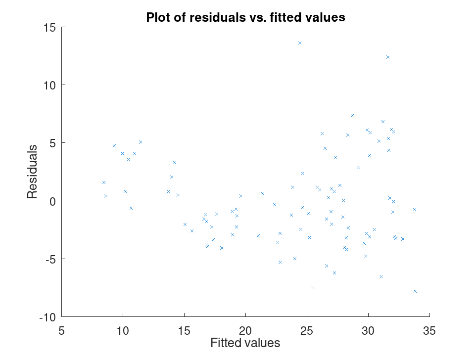
Spotting influential observations with Cook's distance. Sixteen houses are matched by size and age to a sale price, but one house was sold far above what its size and age would predict. After fitting the model, plotDiagnostics with the cookd option highlights that single observation as having outsized influence on the fit.
Size = [80; 95; 110; 120; 65; 140; 100; 130; 90; 150; 75; 105; ...
115; 85; 135; 125];
Age = [5; 10; 3; 8; 20; 2; 15; 6; 12; 1; 18; 9; 4; 14; 7; 11];
Price = [200; 230; 260; 280; 150; 320; 240; 300; 210; 340; 170; ...
250; 270; 190; 500; 290];
X = [Size, Age];
y = Price;
mdl = fitlm (X, y);
plotDiagnostics (mdl, 'cookd')
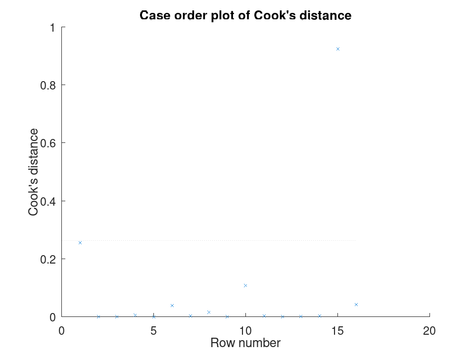
Comparing the size of each predictor's effect, alongside a hypothesis test on the model as a whole. We fit a mileage model on the carsmall data set using weight and horsepower. plotEffects draws each coefficient's estimate with its confidence interval side by side, and coefTest checks whether weight's effect is significantly different from horsepower's.
load carsmall X = [Weight, Horsepower]; y = MPG; mdl = fitlm (X, y);
Visualize the relative size of each predictor's effect.
plotEffects (mdl)
Test whether the two coefficients differ significantly.
H = [0 1 -1]; [p, F, r] = coefTest (mdl, H)
p = 0.073643 F = 3.2759 r = 1
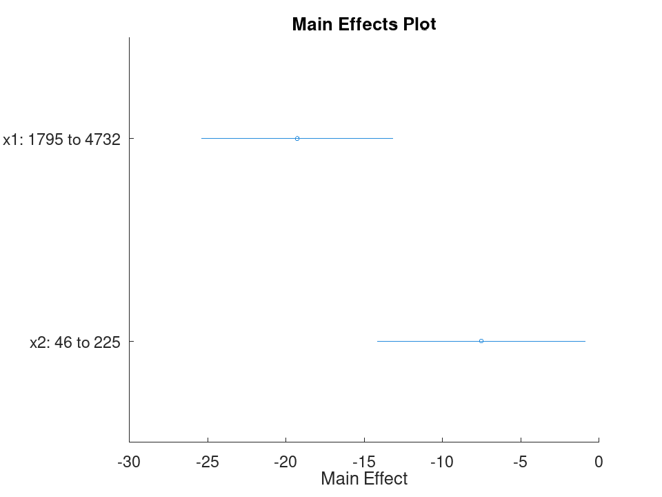
A scalar numeric value equal to the sum of squared deviations of the response from its mean. For a model with an intercept, SST = SSE + SSR. For a robust fit, SST = SSE + SSR rather than the deviation from the mean. For weighted fits, this is the weighted sum of squares. This property is read-only.
Simple linear regression with a single predictor. Ten runners record their weekly training distance and their finish time in a 10k race. We fit a straight line through this data and look at the fitted coefficients, then use predict to estimate the finish time for a runner who trains a distance not in the sample.
Distance = [10; 15; 20; 25; 30; 35; 40; 45; 50; 55]; Time = [58; 55; 52; 50; 47; 45; 43; 41; 40; 38]; X = Distance; y = Time;
Fit the model and inspect the estimated slope and intercept.
mdl = fitlm (X, y)
mdl =
Linear regression model:
y ~ 1 + x1
Estimated Coefficients:
2x4 table
Estimate SE tStat pValue
________ _________ ________ ___________
(Intercept) 61.2 0.654588 93.494 1.91213e-13
x1 -0.44 0.0184226 -23.8836 1.00609e-08
Number of observations: 10, Error degrees of freedom: 8
Root Mean Squared Error: 0.83666
R-squared: 0.986169, Adjusted R-Squared: 0.984441
F-statistic vs. constant model: 570.429, p-value = 1.00609e-08
Predict the finish time for a runner training 32 km per week.
ypred = predict (mdl, 32)
ypred = 47.120
Multiple linear regression with two predictors, followed by a confidence interval on the coefficients. Thirteen coffee shops report their weekly foot traffic and the number of items on their menu, along with weekly revenue. We fit a model with both predictors, then use coefCI to see how precisely each coefficient is estimated.
Traffic = [120; 150; 90; 200; 175; 60; 220; 140; 100; 190; 80; 210; 130];
MenuSize = [8; 12; 6; 15; 10; 5; 18; 9; 7; 14; 6; 16; 11];
Revenue = [1450; 1820; 1010; 2400; 2050; 700; 2650; 1700; 1150; ...
2300; 900; 2500; 1600];
X = [Traffic, MenuSize];
y = Revenue;
Fit the model with both predictors together.
mdl = fitlm (X, y)
mdl =
Linear regression model:
y ~ 1 + x1 + x2
Estimated Coefficients:
3x4 table
Estimate SE tStat pValue
________ ________ ________ ___________
(Intercept) -47.0932 27.3456 -1.72215 0.115771
x1 11.4079 0.616078 18.517 4.55169e-09
x2 11.4344 7.68384 1.48811 0.167562
Number of observations: 13, Error degrees of freedom: 10
Root Mean Squared Error: 32.4551
R-squared: 0.997901, Adjusted R-Squared: 0.997482
F-statistic vs. constant model: 2377.53, p-value = 4.07061e-14
Check how tight the 95% confidence interval is on each coefficient.
ci = coefCI (mdl)
ci =
-108.0231 13.8366
10.0352 12.7806
-5.6862 28.5551
Growing a model with addTerms and predicting with the richer model. We model fuel economy from the carsmall data set using weight and horsepower as main effects only. addTerms then brings in the weight-horsepower interaction without needing to refit by hand, and predict shows how the estimate for a new car changes once that interaction is included.
load carsmall X = [Weight, Horsepower]; y = MPG;
Fit the additive model first.
mdl = fitlm (X, y);
Add the interaction between weight and horsepower.
mdl2 = addTerms (mdl, 'x1:x2');
Compare predictions from both models for the same new car.
Xnew = [3200, 120]; ypred1 = predict (mdl, Xnew)
ypred1 = 21.719
ypred2 = predict (mdl2, Xnew)
ypred2 = 20.416
Simplifying a model with removeTerms and comparing fit quality. We fit the full Hald cement model with all four ingredients, then use removeTerms to drop the weakest predictor and refit automatically. Comparing SSE before and after shows how little explanatory power that ingredient was actually contributing.
load hald X = ingredients; y = heat;
Fit the model with all four ingredients.
mdl = fitlm (X, y);
Drop the third ingredient and refit on the same data.
mdl2 = removeTerms (mdl, 'x3');
Compare how much the error sum of squares changed.
sse_full = mdl.SSE
sse_full = 47.864
sse_reduced = mdl2.SSE
sse_reduced = 47.973
Testing a linear hypothesis and checking residual autocorrelation. Twelve patients are given a drug at different doses over different treatment durations, and a recovery score is recorded. coefTest checks whether the dose and duration coefficients are actually equal, and dwtest separately checks whether the residuals still carry a leftover pattern the model failed to capture.
Dose = [10; 15; 20; 25; 30; 35; 12; 18; 22; 28; 32; 38]; Duration = [5; 7; 9; 11; 13; 15; 6; 8; 10; 12; 14; 16]; Recovery = [42; 48; 55; 60; 68; 74; 45; 52; 58; 65; 71; 78]; X = [Dose, Duration]; y = Recovery; mdl = fitlm (X, y);
Test H0: the Dose and Duration coefficients are equal.
H = [0 1 -1]; [p, F, r] = coefTest (mdl, H)
p = 0.3535 F = 0.9571 r = 1
Check for autocorrelation left over in the residuals.
[pdw, dw] = dwtest (mdl)
pdw = 0.3658 dw = 2.4432
Checking residuals against fitted values. We fit a mileage model on the carsmall data set using weight and horsepower, then plot the raw residuals against the fitted values. A pattern in this plot, rather than a random scatter, would suggest the linear model is missing some curvature in the relationship.
load carsmall X = [Weight, Horsepower]; y = MPG; mdl = fitlm (X, y); plotResiduals (mdl, 'fitted')
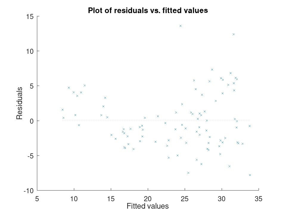
Spotting influential observations with Cook's distance. Sixteen houses are matched by size and age to a sale price, but one house was sold far above what its size and age would predict. After fitting the model, plotDiagnostics with the cookd option highlights that single observation as having outsized influence on the fit.
Size = [80; 95; 110; 120; 65; 140; 100; 130; 90; 150; 75; 105; ...
115; 85; 135; 125];
Age = [5; 10; 3; 8; 20; 2; 15; 6; 12; 1; 18; 9; 4; 14; 7; 11];
Price = [200; 230; 260; 280; 150; 320; 240; 300; 210; 340; 170; ...
250; 270; 190; 500; 290];
X = [Size, Age];
y = Price;
mdl = fitlm (X, y);
plotDiagnostics (mdl, 'cookd')
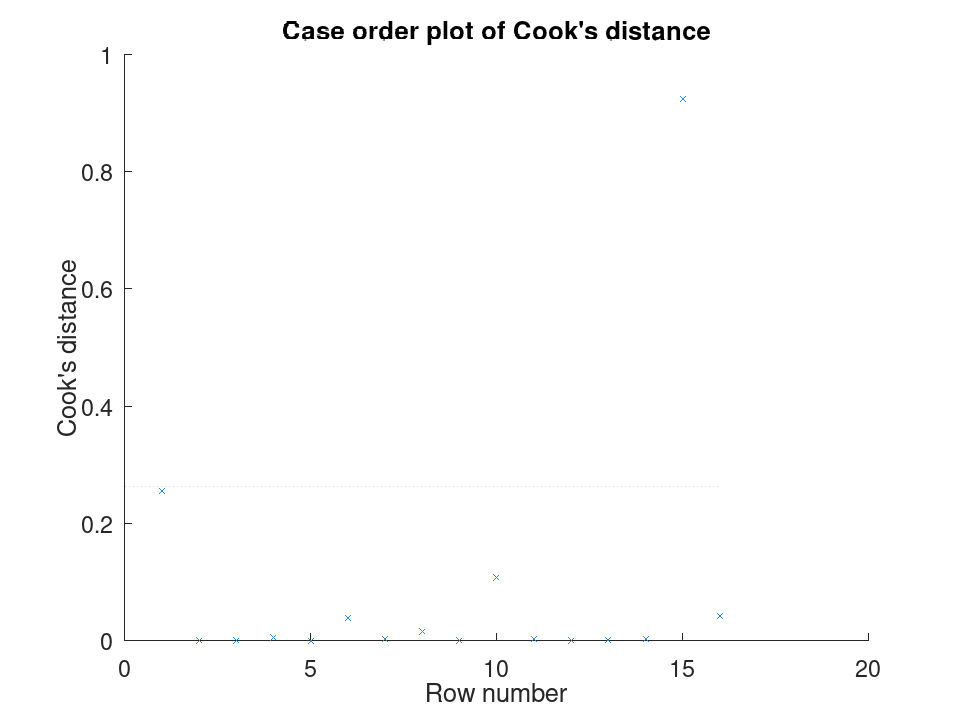
Comparing the size of each predictor's effect, alongside a hypothesis test on the model as a whole. We fit a mileage model on the carsmall data set using weight and horsepower. plotEffects draws each coefficient's estimate with its confidence interval side by side, and coefTest checks whether weight's effect is significantly different from horsepower's.
load carsmall X = [Weight, Horsepower]; y = MPG; mdl = fitlm (X, y);
Visualize the relative size of each predictor's effect.
plotEffects (mdl)
Test whether the two coefficients differ significantly.
H = [0 1 -1]; [p, F, r] = coefTest (mdl, H)
p = 0.073643 F = 3.2759 r = 1
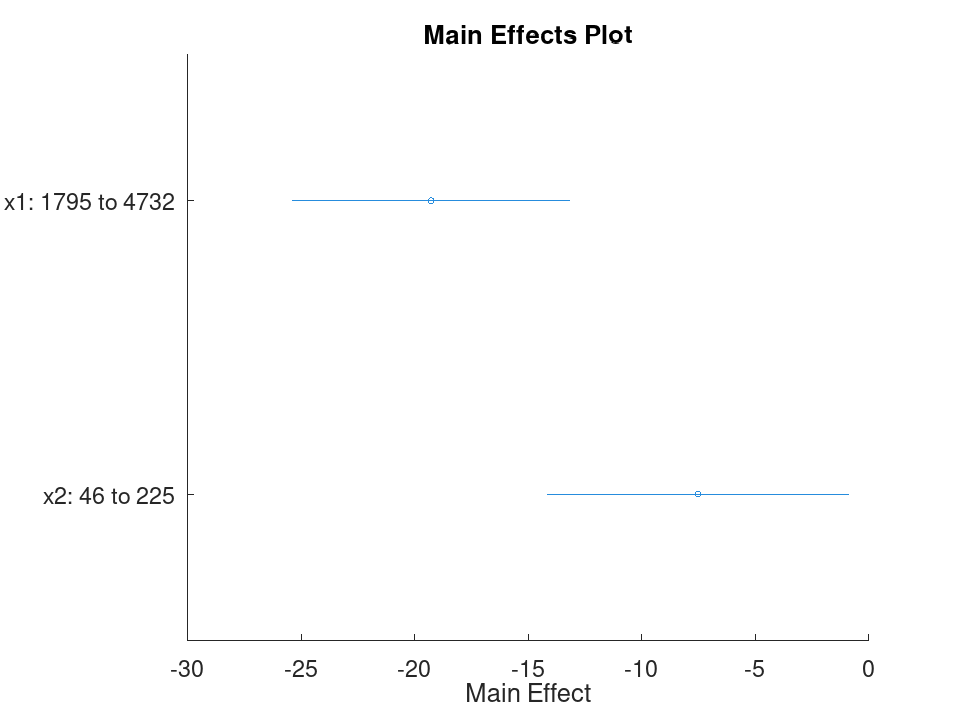
A structure with three fields:
-
WgtFun- robust weighting function name, e.g.'bisquare' -
Tune- tuning constant; empty ifWgtFunis'ols'or a function handle with the default tuning constant -
Weights- vector of final iteration weights; empty for aCompactLinearModelobject
This structure is empty unless the model was fit using robust regression. This property is read-only.
Simple linear regression with a single predictor. Ten runners record their weekly training distance and their finish time in a 10k race. We fit a straight line through this data and look at the fitted coefficients, then use predict to estimate the finish time for a runner who trains a distance not in the sample.
Distance = [10; 15; 20; 25; 30; 35; 40; 45; 50; 55]; Time = [58; 55; 52; 50; 47; 45; 43; 41; 40; 38]; X = Distance; y = Time;
Fit the model and inspect the estimated slope and intercept.
mdl = fitlm (X, y)
mdl =
Linear regression model:
y ~ 1 + x1
Estimated Coefficients:
2x4 table
Estimate SE tStat pValue
________ _________ ________ ___________
(Intercept) 61.2 0.654588 93.494 1.91213e-13
x1 -0.44 0.0184226 -23.8836 1.00609e-08
Number of observations: 10, Error degrees of freedom: 8
Root Mean Squared Error: 0.83666
R-squared: 0.986169, Adjusted R-Squared: 0.984441
F-statistic vs. constant model: 570.429, p-value = 1.00609e-08
Predict the finish time for a runner training 32 km per week.
ypred = predict (mdl, 32)
ypred = 47.120
Multiple linear regression with two predictors, followed by a confidence interval on the coefficients. Thirteen coffee shops report their weekly foot traffic and the number of items on their menu, along with weekly revenue. We fit a model with both predictors, then use coefCI to see how precisely each coefficient is estimated.
Traffic = [120; 150; 90; 200; 175; 60; 220; 140; 100; 190; 80; 210; 130];
MenuSize = [8; 12; 6; 15; 10; 5; 18; 9; 7; 14; 6; 16; 11];
Revenue = [1450; 1820; 1010; 2400; 2050; 700; 2650; 1700; 1150; ...
2300; 900; 2500; 1600];
X = [Traffic, MenuSize];
y = Revenue;
Fit the model with both predictors together.
mdl = fitlm (X, y)
mdl =
Linear regression model:
y ~ 1 + x1 + x2
Estimated Coefficients:
3x4 table
Estimate SE tStat pValue
________ ________ ________ ___________
(Intercept) -47.0932 27.3456 -1.72215 0.115771
x1 11.4079 0.616078 18.517 4.55169e-09
x2 11.4344 7.68384 1.48811 0.167562
Number of observations: 13, Error degrees of freedom: 10
Root Mean Squared Error: 32.4551
R-squared: 0.997901, Adjusted R-Squared: 0.997482
F-statistic vs. constant model: 2377.53, p-value = 4.07061e-14
Check how tight the 95% confidence interval is on each coefficient.
ci = coefCI (mdl)
ci =
-108.0231 13.8366
10.0352 12.7806
-5.6862 28.5551
Growing a model with addTerms and predicting with the richer model. We model fuel economy from the carsmall data set using weight and horsepower as main effects only. addTerms then brings in the weight-horsepower interaction without needing to refit by hand, and predict shows how the estimate for a new car changes once that interaction is included.
load carsmall X = [Weight, Horsepower]; y = MPG;
Fit the additive model first.
mdl = fitlm (X, y);
Add the interaction between weight and horsepower.
mdl2 = addTerms (mdl, 'x1:x2');
Compare predictions from both models for the same new car.
Xnew = [3200, 120]; ypred1 = predict (mdl, Xnew)
ypred1 = 21.719
ypred2 = predict (mdl2, Xnew)
ypred2 = 20.416
Simplifying a model with removeTerms and comparing fit quality. We fit the full Hald cement model with all four ingredients, then use removeTerms to drop the weakest predictor and refit automatically. Comparing SSE before and after shows how little explanatory power that ingredient was actually contributing.
load hald X = ingredients; y = heat;
Fit the model with all four ingredients.
mdl = fitlm (X, y);
Drop the third ingredient and refit on the same data.
mdl2 = removeTerms (mdl, 'x3');
Compare how much the error sum of squares changed.
sse_full = mdl.SSE
sse_full = 47.864
sse_reduced = mdl2.SSE
sse_reduced = 47.973
Testing a linear hypothesis and checking residual autocorrelation. Twelve patients are given a drug at different doses over different treatment durations, and a recovery score is recorded. coefTest checks whether the dose and duration coefficients are actually equal, and dwtest separately checks whether the residuals still carry a leftover pattern the model failed to capture.
Dose = [10; 15; 20; 25; 30; 35; 12; 18; 22; 28; 32; 38]; Duration = [5; 7; 9; 11; 13; 15; 6; 8; 10; 12; 14; 16]; Recovery = [42; 48; 55; 60; 68; 74; 45; 52; 58; 65; 71; 78]; X = [Dose, Duration]; y = Recovery; mdl = fitlm (X, y);
Test H0: the Dose and Duration coefficients are equal.
H = [0 1 -1]; [p, F, r] = coefTest (mdl, H)
p = 0.3535 F = 0.9571 r = 1
Check for autocorrelation left over in the residuals.
[pdw, dw] = dwtest (mdl)
pdw = 0.3658 dw = 2.4432
Checking residuals against fitted values. We fit a mileage model on the carsmall data set using weight and horsepower, then plot the raw residuals against the fitted values. A pattern in this plot, rather than a random scatter, would suggest the linear model is missing some curvature in the relationship.
load carsmall X = [Weight, Horsepower]; y = MPG; mdl = fitlm (X, y); plotResiduals (mdl, 'fitted')
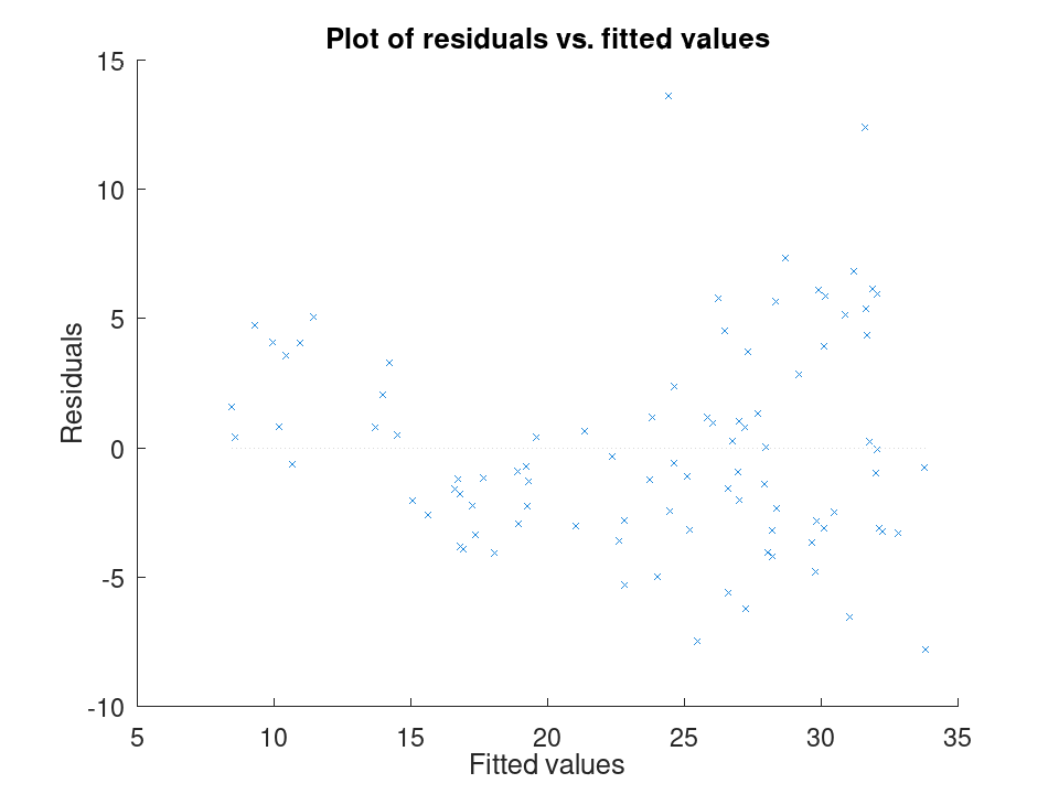
Spotting influential observations with Cook's distance. Sixteen houses are matched by size and age to a sale price, but one house was sold far above what its size and age would predict. After fitting the model, plotDiagnostics with the cookd option highlights that single observation as having outsized influence on the fit.
Size = [80; 95; 110; 120; 65; 140; 100; 130; 90; 150; 75; 105; ...
115; 85; 135; 125];
Age = [5; 10; 3; 8; 20; 2; 15; 6; 12; 1; 18; 9; 4; 14; 7; 11];
Price = [200; 230; 260; 280; 150; 320; 240; 300; 210; 340; 170; ...
250; 270; 190; 500; 290];
X = [Size, Age];
y = Price;
mdl = fitlm (X, y);
plotDiagnostics (mdl, 'cookd')
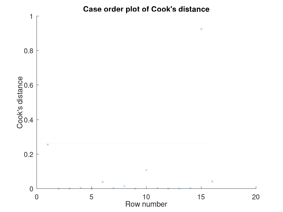
Comparing the size of each predictor's effect, alongside a hypothesis test on the model as a whole. We fit a mileage model on the carsmall data set using weight and horsepower. plotEffects draws each coefficient's estimate with its confidence interval side by side, and coefTest checks whether weight's effect is significantly different from horsepower's.
load carsmall X = [Weight, Horsepower]; y = MPG; mdl = fitlm (X, y);
Visualize the relative size of each predictor's effect.
plotEffects (mdl)
Test whether the two coefficients differ significantly.
H = [0 1 -1]; [p, F, r] = coefTest (mdl, H)
p = 0.073643 F = 3.2759 r = 1
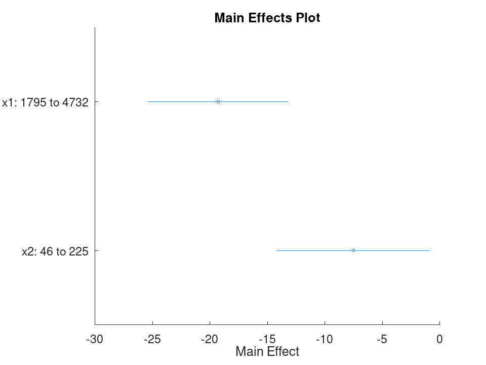
A structure recording the term-selection trace, populated whenever the
model was fit by stepwiselm or improved by step, and
[] otherwise. It has seven fields:
| Field | Contents |
|---|---|
Start | a LinearFormula for the model the search
started from. |
Lower | a LinearFormula for the smallest model
considered; its terms are never removed. |
Upper | a LinearFormula for the largest model
considered. |
Criterion | the selection criterion, such as
'SSE'. |
PEnter | the threshold a term must beat to enter. |
PRemove | the threshold above which a term leaves. |
History | a table with one row per step. |
History carries the columns Action ('Start',
'Add', or 'Remove'), TermName, Terms (the
terms matrix after the step, over the model’s variables), DF (the
coefficient count after the step), and delDF (the change in it,
negative for a removal). The remaining columns follow the criterion:
FStat and pValue under 'SSE', and otherwise a
single column named for the criterion (AIC, BIC,
Rsquared, or AdjRsquared) holding its value after the
step.
The first row is the starting model, named by its right-hand side, and
step appends to the history it inherits rather than starting a
new one. This property is read-only.
Simple linear regression with a single predictor. Ten runners record their weekly training distance and their finish time in a 10k race. We fit a straight line through this data and look at the fitted coefficients, then use predict to estimate the finish time for a runner who trains a distance not in the sample.
Distance = [10; 15; 20; 25; 30; 35; 40; 45; 50; 55]; Time = [58; 55; 52; 50; 47; 45; 43; 41; 40; 38]; X = Distance; y = Time;
Fit the model and inspect the estimated slope and intercept.
mdl = fitlm (X, y)
mdl =
Linear regression model:
y ~ 1 + x1
Estimated Coefficients:
2x4 table
Estimate SE tStat pValue
________ _________ ________ ___________
(Intercept) 61.2 0.654588 93.494 1.91213e-13
x1 -0.44 0.0184226 -23.8836 1.00609e-08
Number of observations: 10, Error degrees of freedom: 8
Root Mean Squared Error: 0.83666
R-squared: 0.986169, Adjusted R-Squared: 0.984441
F-statistic vs. constant model: 570.429, p-value = 1.00609e-08
Predict the finish time for a runner training 32 km per week.
ypred = predict (mdl, 32)
ypred = 47.120
Multiple linear regression with two predictors, followed by a confidence interval on the coefficients. Thirteen coffee shops report their weekly foot traffic and the number of items on their menu, along with weekly revenue. We fit a model with both predictors, then use coefCI to see how precisely each coefficient is estimated.
Traffic = [120; 150; 90; 200; 175; 60; 220; 140; 100; 190; 80; 210; 130];
MenuSize = [8; 12; 6; 15; 10; 5; 18; 9; 7; 14; 6; 16; 11];
Revenue = [1450; 1820; 1010; 2400; 2050; 700; 2650; 1700; 1150; ...
2300; 900; 2500; 1600];
X = [Traffic, MenuSize];
y = Revenue;
Fit the model with both predictors together.
mdl = fitlm (X, y)
mdl =
Linear regression model:
y ~ 1 + x1 + x2
Estimated Coefficients:
3x4 table
Estimate SE tStat pValue
________ ________ ________ ___________
(Intercept) -47.0932 27.3456 -1.72215 0.115771
x1 11.4079 0.616078 18.517 4.55169e-09
x2 11.4344 7.68384 1.48811 0.167562
Number of observations: 13, Error degrees of freedom: 10
Root Mean Squared Error: 32.4551
R-squared: 0.997901, Adjusted R-Squared: 0.997482
F-statistic vs. constant model: 2377.53, p-value = 4.07061e-14
Check how tight the 95% confidence interval is on each coefficient.
ci = coefCI (mdl)
ci =
-108.0231 13.8366
10.0352 12.7806
-5.6862 28.5551
Growing a model with addTerms and predicting with the richer model. We model fuel economy from the carsmall data set using weight and horsepower as main effects only. addTerms then brings in the weight-horsepower interaction without needing to refit by hand, and predict shows how the estimate for a new car changes once that interaction is included.
load carsmall X = [Weight, Horsepower]; y = MPG;
Fit the additive model first.
mdl = fitlm (X, y);
Add the interaction between weight and horsepower.
mdl2 = addTerms (mdl, 'x1:x2');
Compare predictions from both models for the same new car.
Xnew = [3200, 120]; ypred1 = predict (mdl, Xnew)
ypred1 = 21.719
ypred2 = predict (mdl2, Xnew)
ypred2 = 20.416
Simplifying a model with removeTerms and comparing fit quality. We fit the full Hald cement model with all four ingredients, then use removeTerms to drop the weakest predictor and refit automatically. Comparing SSE before and after shows how little explanatory power that ingredient was actually contributing.
load hald X = ingredients; y = heat;
Fit the model with all four ingredients.
mdl = fitlm (X, y);
Drop the third ingredient and refit on the same data.
mdl2 = removeTerms (mdl, 'x3');
Compare how much the error sum of squares changed.
sse_full = mdl.SSE
sse_full = 47.864
sse_reduced = mdl2.SSE
sse_reduced = 47.973
Testing a linear hypothesis and checking residual autocorrelation. Twelve patients are given a drug at different doses over different treatment durations, and a recovery score is recorded. coefTest checks whether the dose and duration coefficients are actually equal, and dwtest separately checks whether the residuals still carry a leftover pattern the model failed to capture.
Dose = [10; 15; 20; 25; 30; 35; 12; 18; 22; 28; 32; 38]; Duration = [5; 7; 9; 11; 13; 15; 6; 8; 10; 12; 14; 16]; Recovery = [42; 48; 55; 60; 68; 74; 45; 52; 58; 65; 71; 78]; X = [Dose, Duration]; y = Recovery; mdl = fitlm (X, y);
Test H0: the Dose and Duration coefficients are equal.
H = [0 1 -1]; [p, F, r] = coefTest (mdl, H)
p = 0.3535 F = 0.9571 r = 1
Check for autocorrelation left over in the residuals.
[pdw, dw] = dwtest (mdl)
pdw = 0.3658 dw = 2.4432
Checking residuals against fitted values. We fit a mileage model on the carsmall data set using weight and horsepower, then plot the raw residuals against the fitted values. A pattern in this plot, rather than a random scatter, would suggest the linear model is missing some curvature in the relationship.
load carsmall X = [Weight, Horsepower]; y = MPG; mdl = fitlm (X, y); plotResiduals (mdl, 'fitted')
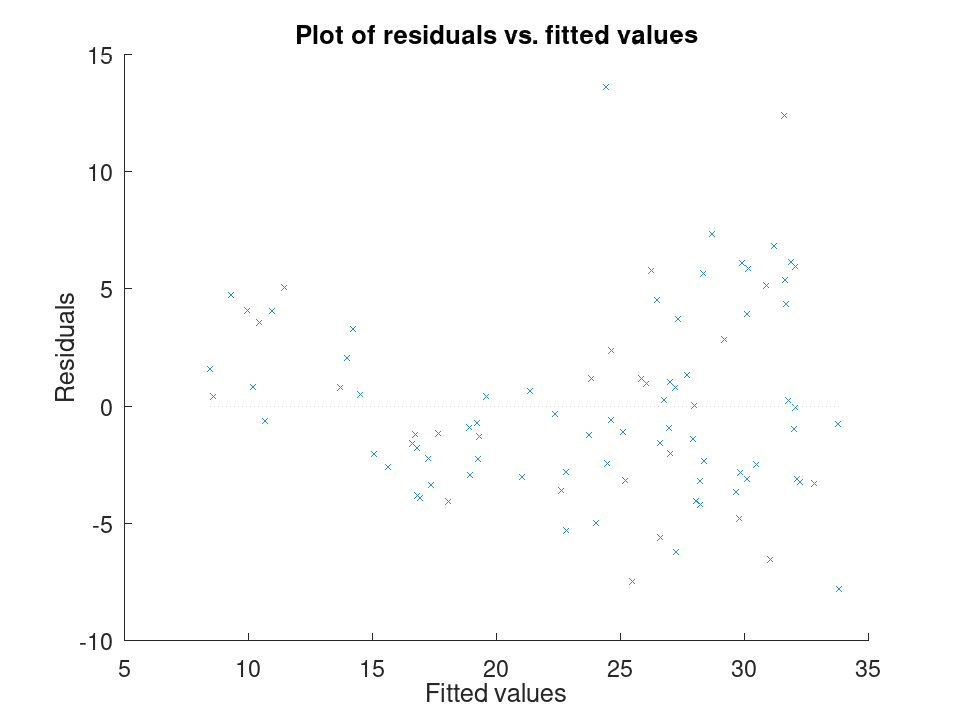
Spotting influential observations with Cook's distance. Sixteen houses are matched by size and age to a sale price, but one house was sold far above what its size and age would predict. After fitting the model, plotDiagnostics with the cookd option highlights that single observation as having outsized influence on the fit.
Size = [80; 95; 110; 120; 65; 140; 100; 130; 90; 150; 75; 105; ...
115; 85; 135; 125];
Age = [5; 10; 3; 8; 20; 2; 15; 6; 12; 1; 18; 9; 4; 14; 7; 11];
Price = [200; 230; 260; 280; 150; 320; 240; 300; 210; 340; 170; ...
250; 270; 190; 500; 290];
X = [Size, Age];
y = Price;
mdl = fitlm (X, y);
plotDiagnostics (mdl, 'cookd')
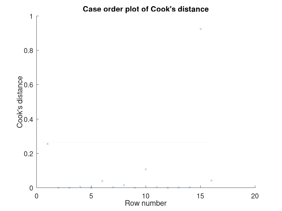
Comparing the size of each predictor's effect, alongside a hypothesis test on the model as a whole. We fit a mileage model on the carsmall data set using weight and horsepower. plotEffects draws each coefficient's estimate with its confidence interval side by side, and coefTest checks whether weight's effect is significantly different from horsepower's.
load carsmall X = [Weight, Horsepower]; y = MPG; mdl = fitlm (X, y);
Visualize the relative size of each predictor's effect.
plotEffects (mdl)
Test whether the two coefficients differ significantly.
H = [0 1 -1]; [p, F, r] = coefTest (mdl, H)
p = 0.073643 F = 3.2759 r = 1
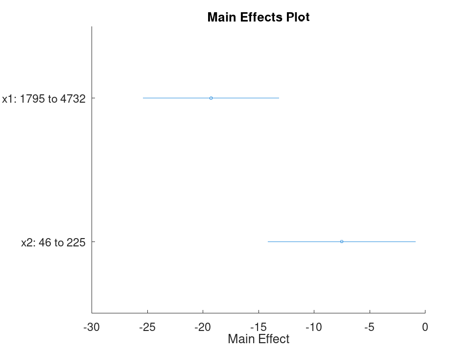
A LinearFormula object representing the model formula, with
properties including ResponseName, LinearPredictor,
PredictorNames, TermNames, HasIntercept,
Terms (the terms matrix), and InModel. Converting it with
char renders the whole formula. This property is read-only.
Simple linear regression with a single predictor. Ten runners record their weekly training distance and their finish time in a 10k race. We fit a straight line through this data and look at the fitted coefficients, then use predict to estimate the finish time for a runner who trains a distance not in the sample.
Distance = [10; 15; 20; 25; 30; 35; 40; 45; 50; 55]; Time = [58; 55; 52; 50; 47; 45; 43; 41; 40; 38]; X = Distance; y = Time;
Fit the model and inspect the estimated slope and intercept.
mdl = fitlm (X, y)
mdl =
Linear regression model:
y ~ 1 + x1
Estimated Coefficients:
2x4 table
Estimate SE tStat pValue
________ _________ ________ ___________
(Intercept) 61.2 0.654588 93.494 1.91213e-13
x1 -0.44 0.0184226 -23.8836 1.00609e-08
Number of observations: 10, Error degrees of freedom: 8
Root Mean Squared Error: 0.83666
R-squared: 0.986169, Adjusted R-Squared: 0.984441
F-statistic vs. constant model: 570.429, p-value = 1.00609e-08
Predict the finish time for a runner training 32 km per week.
ypred = predict (mdl, 32)
ypred = 47.120
Multiple linear regression with two predictors, followed by a confidence interval on the coefficients. Thirteen coffee shops report their weekly foot traffic and the number of items on their menu, along with weekly revenue. We fit a model with both predictors, then use coefCI to see how precisely each coefficient is estimated.
Traffic = [120; 150; 90; 200; 175; 60; 220; 140; 100; 190; 80; 210; 130];
MenuSize = [8; 12; 6; 15; 10; 5; 18; 9; 7; 14; 6; 16; 11];
Revenue = [1450; 1820; 1010; 2400; 2050; 700; 2650; 1700; 1150; ...
2300; 900; 2500; 1600];
X = [Traffic, MenuSize];
y = Revenue;
Fit the model with both predictors together.
mdl = fitlm (X, y)
mdl =
Linear regression model:
y ~ 1 + x1 + x2
Estimated Coefficients:
3x4 table
Estimate SE tStat pValue
________ ________ ________ ___________
(Intercept) -47.0932 27.3456 -1.72215 0.115771
x1 11.4079 0.616078 18.517 4.55169e-09
x2 11.4344 7.68384 1.48811 0.167562
Number of observations: 13, Error degrees of freedom: 10
Root Mean Squared Error: 32.4551
R-squared: 0.997901, Adjusted R-Squared: 0.997482
F-statistic vs. constant model: 2377.53, p-value = 4.07061e-14
Check how tight the 95% confidence interval is on each coefficient.
ci = coefCI (mdl)
ci =
-108.0231 13.8366
10.0352 12.7806
-5.6862 28.5551
Growing a model with addTerms and predicting with the richer model. We model fuel economy from the carsmall data set using weight and horsepower as main effects only. addTerms then brings in the weight-horsepower interaction without needing to refit by hand, and predict shows how the estimate for a new car changes once that interaction is included.
load carsmall X = [Weight, Horsepower]; y = MPG;
Fit the additive model first.
mdl = fitlm (X, y);
Add the interaction between weight and horsepower.
mdl2 = addTerms (mdl, 'x1:x2');
Compare predictions from both models for the same new car.
Xnew = [3200, 120]; ypred1 = predict (mdl, Xnew)
ypred1 = 21.719
ypred2 = predict (mdl2, Xnew)
ypred2 = 20.416
Simplifying a model with removeTerms and comparing fit quality. We fit the full Hald cement model with all four ingredients, then use removeTerms to drop the weakest predictor and refit automatically. Comparing SSE before and after shows how little explanatory power that ingredient was actually contributing.
load hald X = ingredients; y = heat;
Fit the model with all four ingredients.
mdl = fitlm (X, y);
Drop the third ingredient and refit on the same data.
mdl2 = removeTerms (mdl, 'x3');
Compare how much the error sum of squares changed.
sse_full = mdl.SSE
sse_full = 47.864
sse_reduced = mdl2.SSE
sse_reduced = 47.973
Testing a linear hypothesis and checking residual autocorrelation. Twelve patients are given a drug at different doses over different treatment durations, and a recovery score is recorded. coefTest checks whether the dose and duration coefficients are actually equal, and dwtest separately checks whether the residuals still carry a leftover pattern the model failed to capture.
Dose = [10; 15; 20; 25; 30; 35; 12; 18; 22; 28; 32; 38]; Duration = [5; 7; 9; 11; 13; 15; 6; 8; 10; 12; 14; 16]; Recovery = [42; 48; 55; 60; 68; 74; 45; 52; 58; 65; 71; 78]; X = [Dose, Duration]; y = Recovery; mdl = fitlm (X, y);
Test H0: the Dose and Duration coefficients are equal.
H = [0 1 -1]; [p, F, r] = coefTest (mdl, H)
p = 0.3535 F = 0.9571 r = 1
Check for autocorrelation left over in the residuals.
[pdw, dw] = dwtest (mdl)
pdw = 0.3658 dw = 2.4432
Checking residuals against fitted values. We fit a mileage model on the carsmall data set using weight and horsepower, then plot the raw residuals against the fitted values. A pattern in this plot, rather than a random scatter, would suggest the linear model is missing some curvature in the relationship.
load carsmall X = [Weight, Horsepower]; y = MPG; mdl = fitlm (X, y); plotResiduals (mdl, 'fitted')
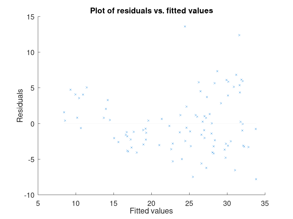
Spotting influential observations with Cook's distance. Sixteen houses are matched by size and age to a sale price, but one house was sold far above what its size and age would predict. After fitting the model, plotDiagnostics with the cookd option highlights that single observation as having outsized influence on the fit.
Size = [80; 95; 110; 120; 65; 140; 100; 130; 90; 150; 75; 105; ...
115; 85; 135; 125];
Age = [5; 10; 3; 8; 20; 2; 15; 6; 12; 1; 18; 9; 4; 14; 7; 11];
Price = [200; 230; 260; 280; 150; 320; 240; 300; 210; 340; 170; ...
250; 270; 190; 500; 290];
X = [Size, Age];
y = Price;
mdl = fitlm (X, y);
plotDiagnostics (mdl, 'cookd')
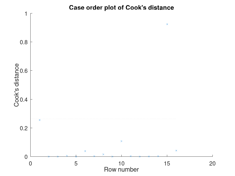
Comparing the size of each predictor's effect, alongside a hypothesis test on the model as a whole. We fit a mileage model on the carsmall data set using weight and horsepower. plotEffects draws each coefficient's estimate with its confidence interval side by side, and coefTest checks whether weight's effect is significantly different from horsepower's.
load carsmall X = [Weight, Horsepower]; y = MPG; mdl = fitlm (X, y);
Visualize the relative size of each predictor's effect.
plotEffects (mdl)
Test whether the two coefficients differ significantly.
H = [0 1 -1]; [p, F, r] = coefTest (mdl, H)
p = 0.073643 F = 3.2759 r = 1
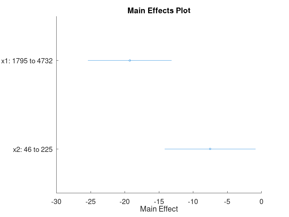
A positive integer giving the number of observations actually used in
fitting. Rows with missing values and rows excluded via the
'Exclude' name-value argument are not counted. This property
is read-only.
Simple linear regression with a single predictor. Ten runners record their weekly training distance and their finish time in a 10k race. We fit a straight line through this data and look at the fitted coefficients, then use predict to estimate the finish time for a runner who trains a distance not in the sample.
Distance = [10; 15; 20; 25; 30; 35; 40; 45; 50; 55]; Time = [58; 55; 52; 50; 47; 45; 43; 41; 40; 38]; X = Distance; y = Time;
Fit the model and inspect the estimated slope and intercept.
mdl = fitlm (X, y)
mdl =
Linear regression model:
y ~ 1 + x1
Estimated Coefficients:
2x4 table
Estimate SE tStat pValue
________ _________ ________ ___________
(Intercept) 61.2 0.654588 93.494 1.91213e-13
x1 -0.44 0.0184226 -23.8836 1.00609e-08
Number of observations: 10, Error degrees of freedom: 8
Root Mean Squared Error: 0.83666
R-squared: 0.986169, Adjusted R-Squared: 0.984441
F-statistic vs. constant model: 570.429, p-value = 1.00609e-08
Predict the finish time for a runner training 32 km per week.
ypred = predict (mdl, 32)
ypred = 47.120
Multiple linear regression with two predictors, followed by a confidence interval on the coefficients. Thirteen coffee shops report their weekly foot traffic and the number of items on their menu, along with weekly revenue. We fit a model with both predictors, then use coefCI to see how precisely each coefficient is estimated.
Traffic = [120; 150; 90; 200; 175; 60; 220; 140; 100; 190; 80; 210; 130];
MenuSize = [8; 12; 6; 15; 10; 5; 18; 9; 7; 14; 6; 16; 11];
Revenue = [1450; 1820; 1010; 2400; 2050; 700; 2650; 1700; 1150; ...
2300; 900; 2500; 1600];
X = [Traffic, MenuSize];
y = Revenue;
Fit the model with both predictors together.
mdl = fitlm (X, y)
mdl =
Linear regression model:
y ~ 1 + x1 + x2
Estimated Coefficients:
3x4 table
Estimate SE tStat pValue
________ ________ ________ ___________
(Intercept) -47.0932 27.3456 -1.72215 0.115771
x1 11.4079 0.616078 18.517 4.55169e-09
x2 11.4344 7.68384 1.48811 0.167562
Number of observations: 13, Error degrees of freedom: 10
Root Mean Squared Error: 32.4551
R-squared: 0.997901, Adjusted R-Squared: 0.997482
F-statistic vs. constant model: 2377.53, p-value = 4.07061e-14
Check how tight the 95% confidence interval is on each coefficient.
ci = coefCI (mdl)
ci =
-108.0231 13.8366
10.0352 12.7806
-5.6862 28.5551
Growing a model with addTerms and predicting with the richer model. We model fuel economy from the carsmall data set using weight and horsepower as main effects only. addTerms then brings in the weight-horsepower interaction without needing to refit by hand, and predict shows how the estimate for a new car changes once that interaction is included.
load carsmall X = [Weight, Horsepower]; y = MPG;
Fit the additive model first.
mdl = fitlm (X, y);
Add the interaction between weight and horsepower.
mdl2 = addTerms (mdl, 'x1:x2');
Compare predictions from both models for the same new car.
Xnew = [3200, 120]; ypred1 = predict (mdl, Xnew)
ypred1 = 21.719
ypred2 = predict (mdl2, Xnew)
ypred2 = 20.416
Simplifying a model with removeTerms and comparing fit quality. We fit the full Hald cement model with all four ingredients, then use removeTerms to drop the weakest predictor and refit automatically. Comparing SSE before and after shows how little explanatory power that ingredient was actually contributing.
load hald X = ingredients; y = heat;
Fit the model with all four ingredients.
mdl = fitlm (X, y);
Drop the third ingredient and refit on the same data.
mdl2 = removeTerms (mdl, 'x3');
Compare how much the error sum of squares changed.
sse_full = mdl.SSE
sse_full = 47.864
sse_reduced = mdl2.SSE
sse_reduced = 47.973
Testing a linear hypothesis and checking residual autocorrelation. Twelve patients are given a drug at different doses over different treatment durations, and a recovery score is recorded. coefTest checks whether the dose and duration coefficients are actually equal, and dwtest separately checks whether the residuals still carry a leftover pattern the model failed to capture.
Dose = [10; 15; 20; 25; 30; 35; 12; 18; 22; 28; 32; 38]; Duration = [5; 7; 9; 11; 13; 15; 6; 8; 10; 12; 14; 16]; Recovery = [42; 48; 55; 60; 68; 74; 45; 52; 58; 65; 71; 78]; X = [Dose, Duration]; y = Recovery; mdl = fitlm (X, y);
Test H0: the Dose and Duration coefficients are equal.
H = [0 1 -1]; [p, F, r] = coefTest (mdl, H)
p = 0.3535 F = 0.9571 r = 1
Check for autocorrelation left over in the residuals.
[pdw, dw] = dwtest (mdl)
pdw = 0.3658 dw = 2.4432
Checking residuals against fitted values. We fit a mileage model on the carsmall data set using weight and horsepower, then plot the raw residuals against the fitted values. A pattern in this plot, rather than a random scatter, would suggest the linear model is missing some curvature in the relationship.
load carsmall X = [Weight, Horsepower]; y = MPG; mdl = fitlm (X, y); plotResiduals (mdl, 'fitted')
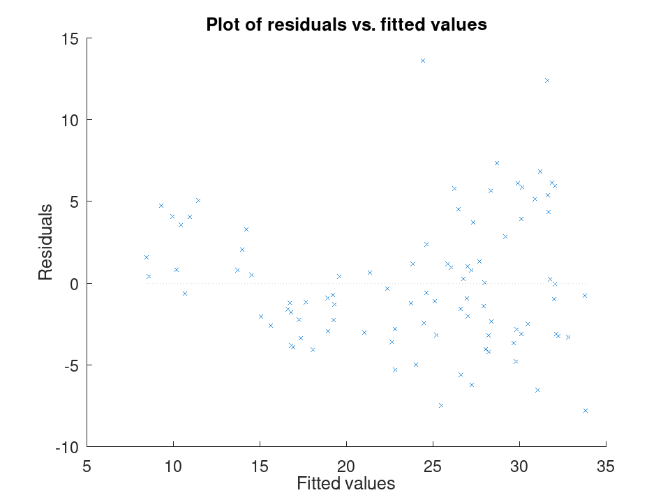
Spotting influential observations with Cook's distance. Sixteen houses are matched by size and age to a sale price, but one house was sold far above what its size and age would predict. After fitting the model, plotDiagnostics with the cookd option highlights that single observation as having outsized influence on the fit.
Size = [80; 95; 110; 120; 65; 140; 100; 130; 90; 150; 75; 105; ...
115; 85; 135; 125];
Age = [5; 10; 3; 8; 20; 2; 15; 6; 12; 1; 18; 9; 4; 14; 7; 11];
Price = [200; 230; 260; 280; 150; 320; 240; 300; 210; 340; 170; ...
250; 270; 190; 500; 290];
X = [Size, Age];
y = Price;
mdl = fitlm (X, y);
plotDiagnostics (mdl, 'cookd')
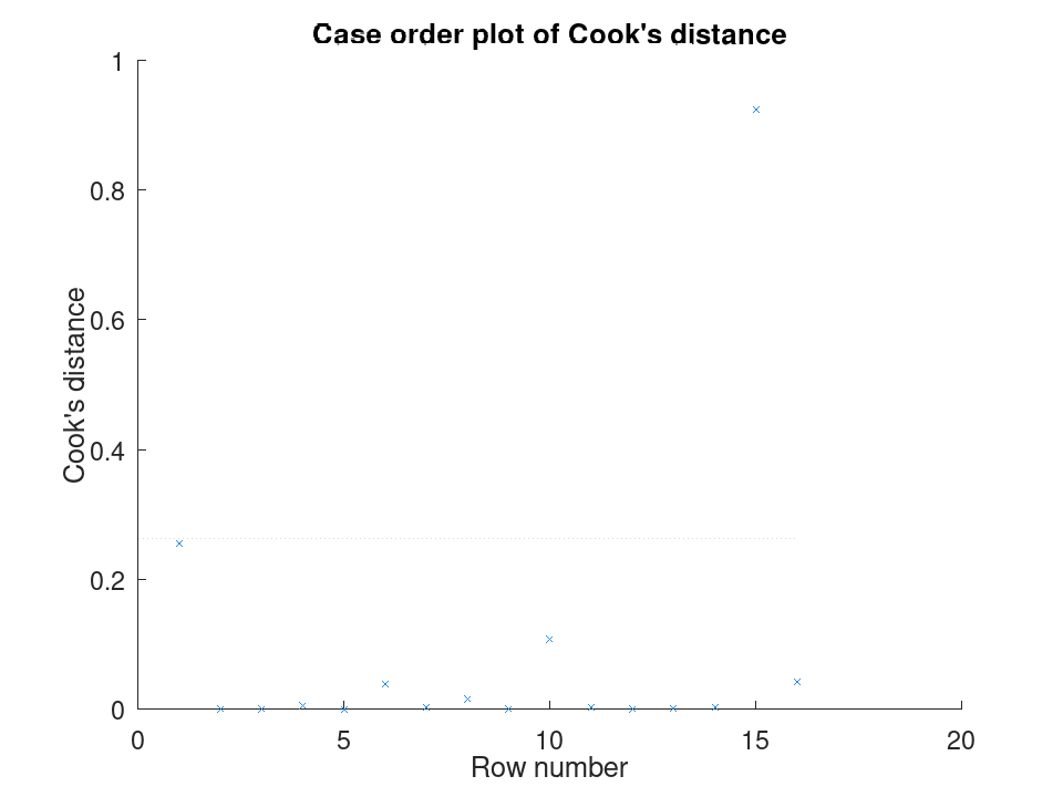
Comparing the size of each predictor's effect, alongside a hypothesis test on the model as a whole. We fit a mileage model on the carsmall data set using weight and horsepower. plotEffects draws each coefficient's estimate with its confidence interval side by side, and coefTest checks whether weight's effect is significantly different from horsepower's.
load carsmall X = [Weight, Horsepower]; y = MPG; mdl = fitlm (X, y);
Visualize the relative size of each predictor's effect.
plotEffects (mdl)
Test whether the two coefficients differ significantly.
H = [0 1 -1]; [p, F, r] = coefTest (mdl, H)
p = 0.073643 F = 3.2759 r = 1
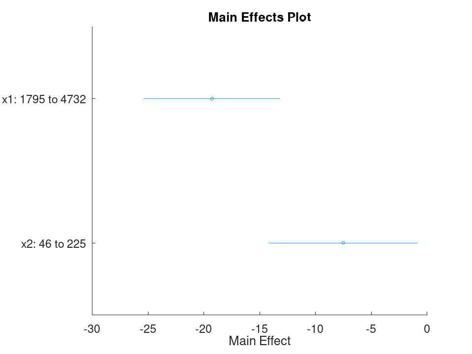
A positive integer giving the number of predictor variables used to fit the model. This property is read-only.
Simple linear regression with a single predictor. Ten runners record their weekly training distance and their finish time in a 10k race. We fit a straight line through this data and look at the fitted coefficients, then use predict to estimate the finish time for a runner who trains a distance not in the sample.
Distance = [10; 15; 20; 25; 30; 35; 40; 45; 50; 55]; Time = [58; 55; 52; 50; 47; 45; 43; 41; 40; 38]; X = Distance; y = Time;
Fit the model and inspect the estimated slope and intercept.
mdl = fitlm (X, y)
mdl =
Linear regression model:
y ~ 1 + x1
Estimated Coefficients:
2x4 table
Estimate SE tStat pValue
________ _________ ________ ___________
(Intercept) 61.2 0.654588 93.494 1.91213e-13
x1 -0.44 0.0184226 -23.8836 1.00609e-08
Number of observations: 10, Error degrees of freedom: 8
Root Mean Squared Error: 0.83666
R-squared: 0.986169, Adjusted R-Squared: 0.984441
F-statistic vs. constant model: 570.429, p-value = 1.00609e-08
Predict the finish time for a runner training 32 km per week.
ypred = predict (mdl, 32)
ypred = 47.120
Multiple linear regression with two predictors, followed by a confidence interval on the coefficients. Thirteen coffee shops report their weekly foot traffic and the number of items on their menu, along with weekly revenue. We fit a model with both predictors, then use coefCI to see how precisely each coefficient is estimated.
Traffic = [120; 150; 90; 200; 175; 60; 220; 140; 100; 190; 80; 210; 130];
MenuSize = [8; 12; 6; 15; 10; 5; 18; 9; 7; 14; 6; 16; 11];
Revenue = [1450; 1820; 1010; 2400; 2050; 700; 2650; 1700; 1150; ...
2300; 900; 2500; 1600];
X = [Traffic, MenuSize];
y = Revenue;
Fit the model with both predictors together.
mdl = fitlm (X, y)
mdl =
Linear regression model:
y ~ 1 + x1 + x2
Estimated Coefficients:
3x4 table
Estimate SE tStat pValue
________ ________ ________ ___________
(Intercept) -47.0932 27.3456 -1.72215 0.115771
x1 11.4079 0.616078 18.517 4.55169e-09
x2 11.4344 7.68384 1.48811 0.167562
Number of observations: 13, Error degrees of freedom: 10
Root Mean Squared Error: 32.4551
R-squared: 0.997901, Adjusted R-Squared: 0.997482
F-statistic vs. constant model: 2377.53, p-value = 4.07061e-14
Check how tight the 95% confidence interval is on each coefficient.
ci = coefCI (mdl)
ci =
-108.0231 13.8366
10.0352 12.7806
-5.6862 28.5551
Growing a model with addTerms and predicting with the richer model. We model fuel economy from the carsmall data set using weight and horsepower as main effects only. addTerms then brings in the weight-horsepower interaction without needing to refit by hand, and predict shows how the estimate for a new car changes once that interaction is included.
load carsmall X = [Weight, Horsepower]; y = MPG;
Fit the additive model first.
mdl = fitlm (X, y);
Add the interaction between weight and horsepower.
mdl2 = addTerms (mdl, 'x1:x2');
Compare predictions from both models for the same new car.
Xnew = [3200, 120]; ypred1 = predict (mdl, Xnew)
ypred1 = 21.719
ypred2 = predict (mdl2, Xnew)
ypred2 = 20.416
Simplifying a model with removeTerms and comparing fit quality. We fit the full Hald cement model with all four ingredients, then use removeTerms to drop the weakest predictor and refit automatically. Comparing SSE before and after shows how little explanatory power that ingredient was actually contributing.
load hald X = ingredients; y = heat;
Fit the model with all four ingredients.
mdl = fitlm (X, y);
Drop the third ingredient and refit on the same data.
mdl2 = removeTerms (mdl, 'x3');
Compare how much the error sum of squares changed.
sse_full = mdl.SSE
sse_full = 47.864
sse_reduced = mdl2.SSE
sse_reduced = 47.973
Testing a linear hypothesis and checking residual autocorrelation. Twelve patients are given a drug at different doses over different treatment durations, and a recovery score is recorded. coefTest checks whether the dose and duration coefficients are actually equal, and dwtest separately checks whether the residuals still carry a leftover pattern the model failed to capture.
Dose = [10; 15; 20; 25; 30; 35; 12; 18; 22; 28; 32; 38]; Duration = [5; 7; 9; 11; 13; 15; 6; 8; 10; 12; 14; 16]; Recovery = [42; 48; 55; 60; 68; 74; 45; 52; 58; 65; 71; 78]; X = [Dose, Duration]; y = Recovery; mdl = fitlm (X, y);
Test H0: the Dose and Duration coefficients are equal.
H = [0 1 -1]; [p, F, r] = coefTest (mdl, H)
p = 0.3535 F = 0.9571 r = 1
Check for autocorrelation left over in the residuals.
[pdw, dw] = dwtest (mdl)
pdw = 0.3658 dw = 2.4432
Checking residuals against fitted values. We fit a mileage model on the carsmall data set using weight and horsepower, then plot the raw residuals against the fitted values. A pattern in this plot, rather than a random scatter, would suggest the linear model is missing some curvature in the relationship.
load carsmall X = [Weight, Horsepower]; y = MPG; mdl = fitlm (X, y); plotResiduals (mdl, 'fitted')
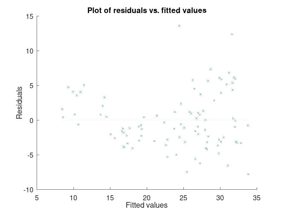
Spotting influential observations with Cook's distance. Sixteen houses are matched by size and age to a sale price, but one house was sold far above what its size and age would predict. After fitting the model, plotDiagnostics with the cookd option highlights that single observation as having outsized influence on the fit.
Size = [80; 95; 110; 120; 65; 140; 100; 130; 90; 150; 75; 105; ...
115; 85; 135; 125];
Age = [5; 10; 3; 8; 20; 2; 15; 6; 12; 1; 18; 9; 4; 14; 7; 11];
Price = [200; 230; 260; 280; 150; 320; 240; 300; 210; 340; 170; ...
250; 270; 190; 500; 290];
X = [Size, Age];
y = Price;
mdl = fitlm (X, y);
plotDiagnostics (mdl, 'cookd')
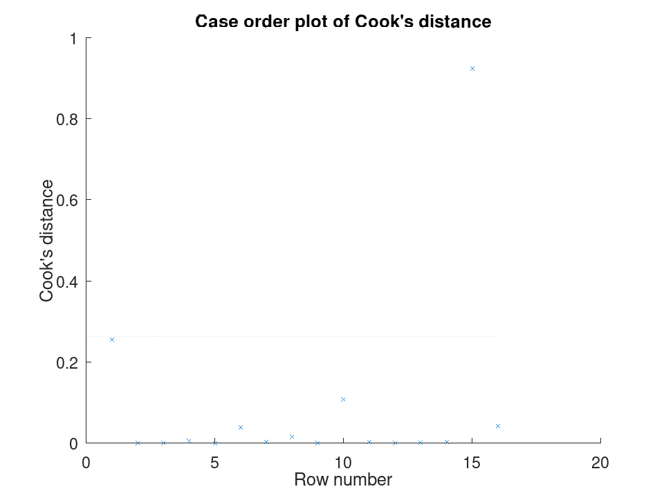
Comparing the size of each predictor's effect, alongside a hypothesis test on the model as a whole. We fit a mileage model on the carsmall data set using weight and horsepower. plotEffects draws each coefficient's estimate with its confidence interval side by side, and coefTest checks whether weight's effect is significantly different from horsepower's.
load carsmall X = [Weight, Horsepower]; y = MPG; mdl = fitlm (X, y);
Visualize the relative size of each predictor's effect.
plotEffects (mdl)
Test whether the two coefficients differ significantly.
H = [0 1 -1]; [p, F, r] = coefTest (mdl, H)
p = 0.073643 F = 3.2759 r = 1
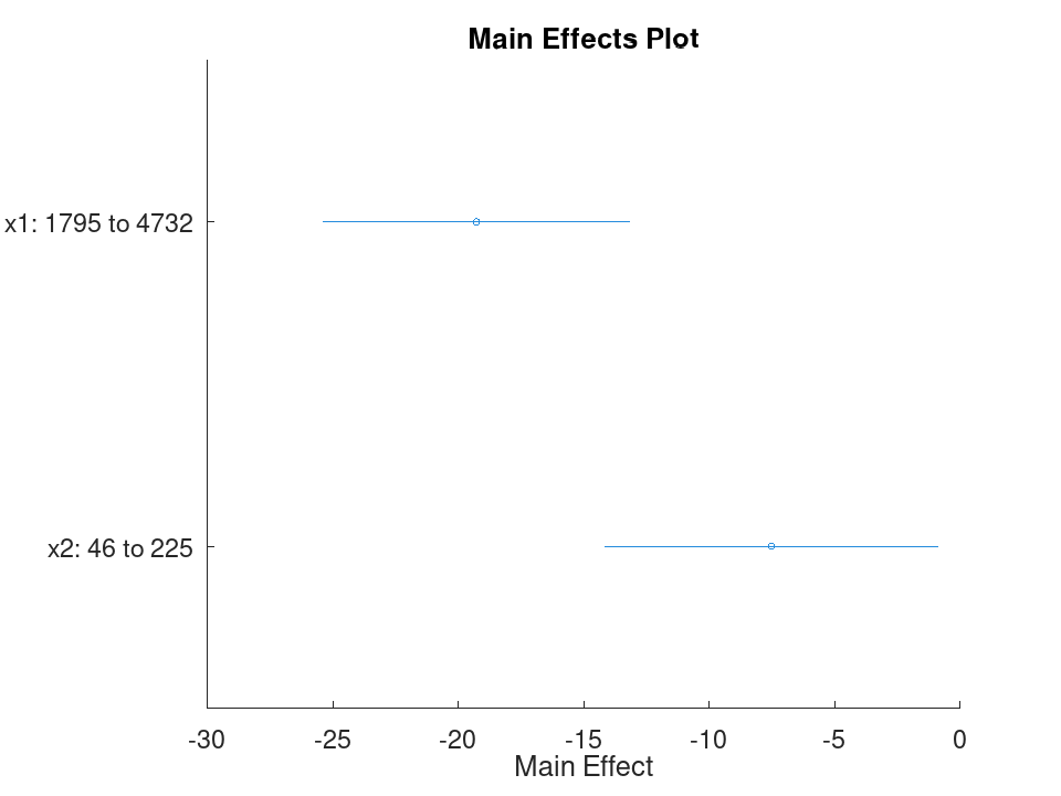
A positive integer giving the total number of variables in the input data, counting predictors, the response, and any unused columns. This property is read-only.
Simple linear regression with a single predictor. Ten runners record their weekly training distance and their finish time in a 10k race. We fit a straight line through this data and look at the fitted coefficients, then use predict to estimate the finish time for a runner who trains a distance not in the sample.
Distance = [10; 15; 20; 25; 30; 35; 40; 45; 50; 55]; Time = [58; 55; 52; 50; 47; 45; 43; 41; 40; 38]; X = Distance; y = Time;
Fit the model and inspect the estimated slope and intercept.
mdl = fitlm (X, y)
mdl =
Linear regression model:
y ~ 1 + x1
Estimated Coefficients:
2x4 table
Estimate SE tStat pValue
________ _________ ________ ___________
(Intercept) 61.2 0.654588 93.494 1.91213e-13
x1 -0.44 0.0184226 -23.8836 1.00609e-08
Number of observations: 10, Error degrees of freedom: 8
Root Mean Squared Error: 0.83666
R-squared: 0.986169, Adjusted R-Squared: 0.984441
F-statistic vs. constant model: 570.429, p-value = 1.00609e-08
Predict the finish time for a runner training 32 km per week.
ypred = predict (mdl, 32)
ypred = 47.120
Multiple linear regression with two predictors, followed by a confidence interval on the coefficients. Thirteen coffee shops report their weekly foot traffic and the number of items on their menu, along with weekly revenue. We fit a model with both predictors, then use coefCI to see how precisely each coefficient is estimated.
Traffic = [120; 150; 90; 200; 175; 60; 220; 140; 100; 190; 80; 210; 130];
MenuSize = [8; 12; 6; 15; 10; 5; 18; 9; 7; 14; 6; 16; 11];
Revenue = [1450; 1820; 1010; 2400; 2050; 700; 2650; 1700; 1150; ...
2300; 900; 2500; 1600];
X = [Traffic, MenuSize];
y = Revenue;
Fit the model with both predictors together.
mdl = fitlm (X, y)
mdl =
Linear regression model:
y ~ 1 + x1 + x2
Estimated Coefficients:
3x4 table
Estimate SE tStat pValue
________ ________ ________ ___________
(Intercept) -47.0932 27.3456 -1.72215 0.115771
x1 11.4079 0.616078 18.517 4.55169e-09
x2 11.4344 7.68384 1.48811 0.167562
Number of observations: 13, Error degrees of freedom: 10
Root Mean Squared Error: 32.4551
R-squared: 0.997901, Adjusted R-Squared: 0.997482
F-statistic vs. constant model: 2377.53, p-value = 4.07061e-14
Check how tight the 95% confidence interval is on each coefficient.
ci = coefCI (mdl)
ci =
-108.0231 13.8366
10.0352 12.7806
-5.6862 28.5551
Growing a model with addTerms and predicting with the richer model. We model fuel economy from the carsmall data set using weight and horsepower as main effects only. addTerms then brings in the weight-horsepower interaction without needing to refit by hand, and predict shows how the estimate for a new car changes once that interaction is included.
load carsmall X = [Weight, Horsepower]; y = MPG;
Fit the additive model first.
mdl = fitlm (X, y);
Add the interaction between weight and horsepower.
mdl2 = addTerms (mdl, 'x1:x2');
Compare predictions from both models for the same new car.
Xnew = [3200, 120]; ypred1 = predict (mdl, Xnew)
ypred1 = 21.719
ypred2 = predict (mdl2, Xnew)
ypred2 = 20.416
Simplifying a model with removeTerms and comparing fit quality. We fit the full Hald cement model with all four ingredients, then use removeTerms to drop the weakest predictor and refit automatically. Comparing SSE before and after shows how little explanatory power that ingredient was actually contributing.
load hald X = ingredients; y = heat;
Fit the model with all four ingredients.
mdl = fitlm (X, y);
Drop the third ingredient and refit on the same data.
mdl2 = removeTerms (mdl, 'x3');
Compare how much the error sum of squares changed.
sse_full = mdl.SSE
sse_full = 47.864
sse_reduced = mdl2.SSE
sse_reduced = 47.973
Testing a linear hypothesis and checking residual autocorrelation. Twelve patients are given a drug at different doses over different treatment durations, and a recovery score is recorded. coefTest checks whether the dose and duration coefficients are actually equal, and dwtest separately checks whether the residuals still carry a leftover pattern the model failed to capture.
Dose = [10; 15; 20; 25; 30; 35; 12; 18; 22; 28; 32; 38]; Duration = [5; 7; 9; 11; 13; 15; 6; 8; 10; 12; 14; 16]; Recovery = [42; 48; 55; 60; 68; 74; 45; 52; 58; 65; 71; 78]; X = [Dose, Duration]; y = Recovery; mdl = fitlm (X, y);
Test H0: the Dose and Duration coefficients are equal.
H = [0 1 -1]; [p, F, r] = coefTest (mdl, H)
p = 0.3535 F = 0.9571 r = 1
Check for autocorrelation left over in the residuals.
[pdw, dw] = dwtest (mdl)
pdw = 0.3658 dw = 2.4432
Checking residuals against fitted values. We fit a mileage model on the carsmall data set using weight and horsepower, then plot the raw residuals against the fitted values. A pattern in this plot, rather than a random scatter, would suggest the linear model is missing some curvature in the relationship.
load carsmall X = [Weight, Horsepower]; y = MPG; mdl = fitlm (X, y); plotResiduals (mdl, 'fitted')
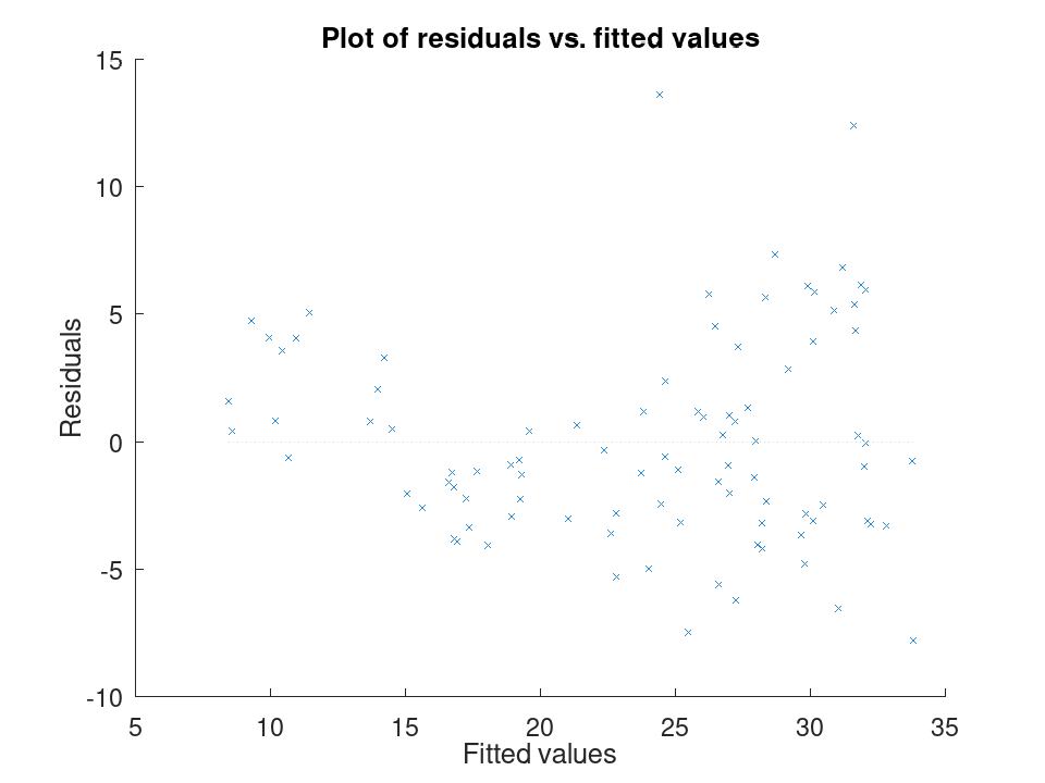
Spotting influential observations with Cook's distance. Sixteen houses are matched by size and age to a sale price, but one house was sold far above what its size and age would predict. After fitting the model, plotDiagnostics with the cookd option highlights that single observation as having outsized influence on the fit.
Size = [80; 95; 110; 120; 65; 140; 100; 130; 90; 150; 75; 105; ...
115; 85; 135; 125];
Age = [5; 10; 3; 8; 20; 2; 15; 6; 12; 1; 18; 9; 4; 14; 7; 11];
Price = [200; 230; 260; 280; 150; 320; 240; 300; 210; 340; 170; ...
250; 270; 190; 500; 290];
X = [Size, Age];
y = Price;
mdl = fitlm (X, y);
plotDiagnostics (mdl, 'cookd')
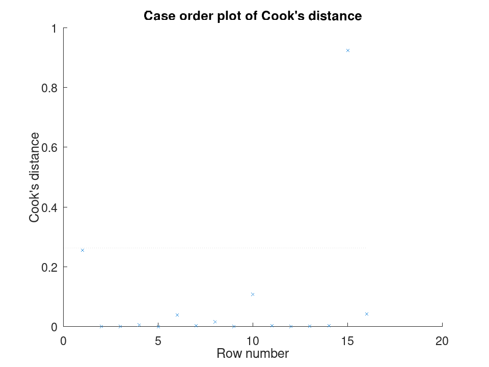
Comparing the size of each predictor's effect, alongside a hypothesis test on the model as a whole. We fit a mileage model on the carsmall data set using weight and horsepower. plotEffects draws each coefficient's estimate with its confidence interval side by side, and coefTest checks whether weight's effect is significantly different from horsepower's.
load carsmall X = [Weight, Horsepower]; y = MPG; mdl = fitlm (X, y);
Visualize the relative size of each predictor's effect.
plotEffects (mdl)
Test whether the two coefficients differ significantly.
H = [0 1 -1]; [p, F, r] = coefTest (mdl, H)
p = 0.073643 F = 3.2759 r = 1
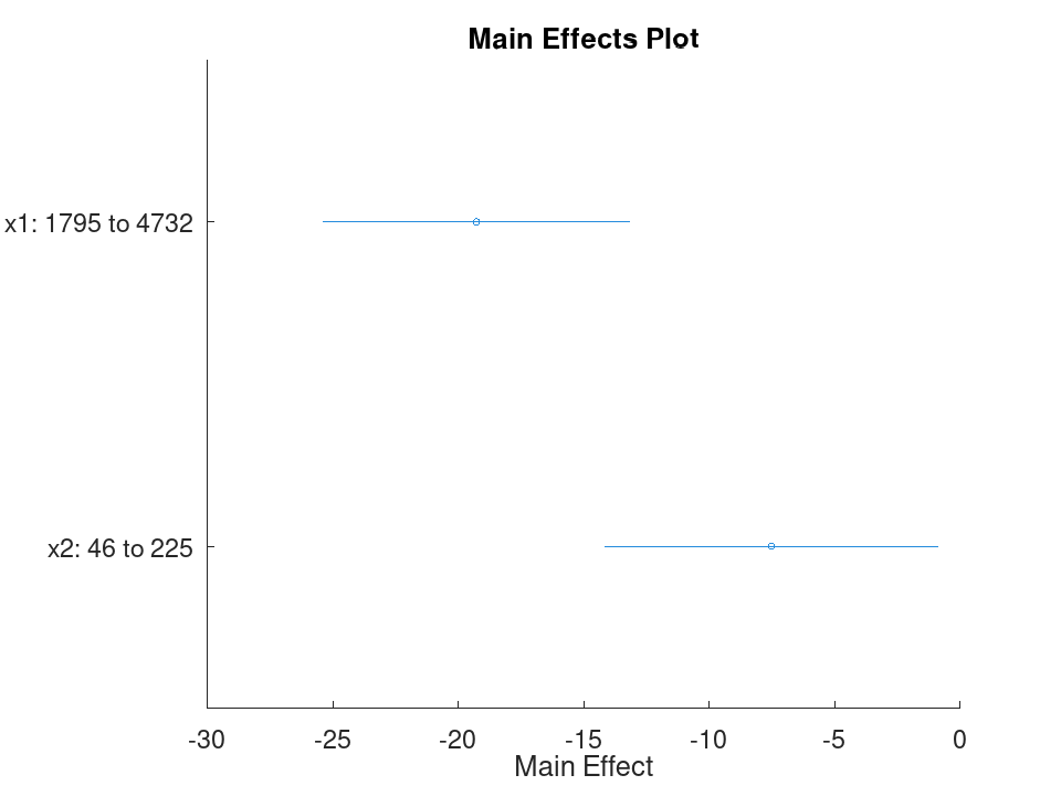
An n-by-4 table where n is the total number of rows in the input data. The four columns are:
-
Weights- observation weight, default is 1 -
Excluded- logical; true if excluded via the'Exclude'argument -
Missing- logical; true if the row contains anyNaNvalue -
Subset- logical; true if the observation was used in the fit, i.e. not excluded and not missing
This property is read-only.
Simple linear regression with a single predictor. Ten runners record their weekly training distance and their finish time in a 10k race. We fit a straight line through this data and look at the fitted coefficients, then use predict to estimate the finish time for a runner who trains a distance not in the sample.
Distance = [10; 15; 20; 25; 30; 35; 40; 45; 50; 55]; Time = [58; 55; 52; 50; 47; 45; 43; 41; 40; 38]; X = Distance; y = Time;
Fit the model and inspect the estimated slope and intercept.
mdl = fitlm (X, y)
mdl =
Linear regression model:
y ~ 1 + x1
Estimated Coefficients:
2x4 table
Estimate SE tStat pValue
________ _________ ________ ___________
(Intercept) 61.2 0.654588 93.494 1.91213e-13
x1 -0.44 0.0184226 -23.8836 1.00609e-08
Number of observations: 10, Error degrees of freedom: 8
Root Mean Squared Error: 0.83666
R-squared: 0.986169, Adjusted R-Squared: 0.984441
F-statistic vs. constant model: 570.429, p-value = 1.00609e-08
Predict the finish time for a runner training 32 km per week.
ypred = predict (mdl, 32)
ypred = 47.120
Multiple linear regression with two predictors, followed by a confidence interval on the coefficients. Thirteen coffee shops report their weekly foot traffic and the number of items on their menu, along with weekly revenue. We fit a model with both predictors, then use coefCI to see how precisely each coefficient is estimated.
Traffic = [120; 150; 90; 200; 175; 60; 220; 140; 100; 190; 80; 210; 130];
MenuSize = [8; 12; 6; 15; 10; 5; 18; 9; 7; 14; 6; 16; 11];
Revenue = [1450; 1820; 1010; 2400; 2050; 700; 2650; 1700; 1150; ...
2300; 900; 2500; 1600];
X = [Traffic, MenuSize];
y = Revenue;
Fit the model with both predictors together.
mdl = fitlm (X, y)
mdl =
Linear regression model:
y ~ 1 + x1 + x2
Estimated Coefficients:
3x4 table
Estimate SE tStat pValue
________ ________ ________ ___________
(Intercept) -47.0932 27.3456 -1.72215 0.115771
x1 11.4079 0.616078 18.517 4.55169e-09
x2 11.4344 7.68384 1.48811 0.167562
Number of observations: 13, Error degrees of freedom: 10
Root Mean Squared Error: 32.4551
R-squared: 0.997901, Adjusted R-Squared: 0.997482
F-statistic vs. constant model: 2377.53, p-value = 4.07061e-14
Check how tight the 95% confidence interval is on each coefficient.
ci = coefCI (mdl)
ci =
-108.0231 13.8366
10.0352 12.7806
-5.6862 28.5551
Growing a model with addTerms and predicting with the richer model. We model fuel economy from the carsmall data set using weight and horsepower as main effects only. addTerms then brings in the weight-horsepower interaction without needing to refit by hand, and predict shows how the estimate for a new car changes once that interaction is included.
load carsmall X = [Weight, Horsepower]; y = MPG;
Fit the additive model first.
mdl = fitlm (X, y);
Add the interaction between weight and horsepower.
mdl2 = addTerms (mdl, 'x1:x2');
Compare predictions from both models for the same new car.
Xnew = [3200, 120]; ypred1 = predict (mdl, Xnew)
ypred1 = 21.719
ypred2 = predict (mdl2, Xnew)
ypred2 = 20.416
Simplifying a model with removeTerms and comparing fit quality. We fit the full Hald cement model with all four ingredients, then use removeTerms to drop the weakest predictor and refit automatically. Comparing SSE before and after shows how little explanatory power that ingredient was actually contributing.
load hald X = ingredients; y = heat;
Fit the model with all four ingredients.
mdl = fitlm (X, y);
Drop the third ingredient and refit on the same data.
mdl2 = removeTerms (mdl, 'x3');
Compare how much the error sum of squares changed.
sse_full = mdl.SSE
sse_full = 47.864
sse_reduced = mdl2.SSE
sse_reduced = 47.973
Testing a linear hypothesis and checking residual autocorrelation. Twelve patients are given a drug at different doses over different treatment durations, and a recovery score is recorded. coefTest checks whether the dose and duration coefficients are actually equal, and dwtest separately checks whether the residuals still carry a leftover pattern the model failed to capture.
Dose = [10; 15; 20; 25; 30; 35; 12; 18; 22; 28; 32; 38]; Duration = [5; 7; 9; 11; 13; 15; 6; 8; 10; 12; 14; 16]; Recovery = [42; 48; 55; 60; 68; 74; 45; 52; 58; 65; 71; 78]; X = [Dose, Duration]; y = Recovery; mdl = fitlm (X, y);
Test H0: the Dose and Duration coefficients are equal.
H = [0 1 -1]; [p, F, r] = coefTest (mdl, H)
p = 0.3535 F = 0.9571 r = 1
Check for autocorrelation left over in the residuals.
[pdw, dw] = dwtest (mdl)
pdw = 0.3658 dw = 2.4432
Checking residuals against fitted values. We fit a mileage model on the carsmall data set using weight and horsepower, then plot the raw residuals against the fitted values. A pattern in this plot, rather than a random scatter, would suggest the linear model is missing some curvature in the relationship.
load carsmall X = [Weight, Horsepower]; y = MPG; mdl = fitlm (X, y); plotResiduals (mdl, 'fitted')
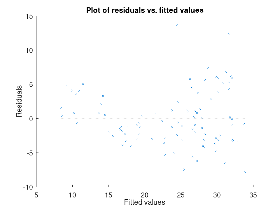
Spotting influential observations with Cook's distance. Sixteen houses are matched by size and age to a sale price, but one house was sold far above what its size and age would predict. After fitting the model, plotDiagnostics with the cookd option highlights that single observation as having outsized influence on the fit.
Size = [80; 95; 110; 120; 65; 140; 100; 130; 90; 150; 75; 105; ...
115; 85; 135; 125];
Age = [5; 10; 3; 8; 20; 2; 15; 6; 12; 1; 18; 9; 4; 14; 7; 11];
Price = [200; 230; 260; 280; 150; 320; 240; 300; 210; 340; 170; ...
250; 270; 190; 500; 290];
X = [Size, Age];
y = Price;
mdl = fitlm (X, y);
plotDiagnostics (mdl, 'cookd')
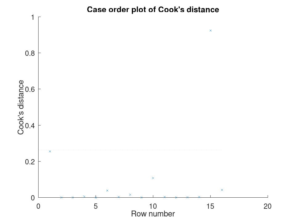
Comparing the size of each predictor's effect, alongside a hypothesis test on the model as a whole. We fit a mileage model on the carsmall data set using weight and horsepower. plotEffects draws each coefficient's estimate with its confidence interval side by side, and coefTest checks whether weight's effect is significantly different from horsepower's.
load carsmall X = [Weight, Horsepower]; y = MPG; mdl = fitlm (X, y);
Visualize the relative size of each predictor's effect.
plotEffects (mdl)
Test whether the two coefficients differ significantly.
H = [0 1 -1]; [p, F, r] = coefTest (mdl, H)
p = 0.073643 F = 3.2759 r = 1
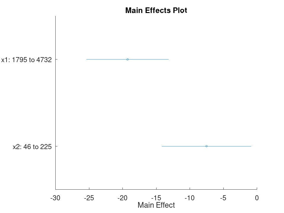
A cell array of character vectors containing the names of the observations. If the fit was based on a table that has row names, this property holds those names. Otherwise it is an empty cell array. This property is read-only.
Simple linear regression with a single predictor. Ten runners record their weekly training distance and their finish time in a 10k race. We fit a straight line through this data and look at the fitted coefficients, then use predict to estimate the finish time for a runner who trains a distance not in the sample.
Distance = [10; 15; 20; 25; 30; 35; 40; 45; 50; 55]; Time = [58; 55; 52; 50; 47; 45; 43; 41; 40; 38]; X = Distance; y = Time;
Fit the model and inspect the estimated slope and intercept.
mdl = fitlm (X, y)
mdl =
Linear regression model:
y ~ 1 + x1
Estimated Coefficients:
2x4 table
Estimate SE tStat pValue
________ _________ ________ ___________
(Intercept) 61.2 0.654588 93.494 1.91213e-13
x1 -0.44 0.0184226 -23.8836 1.00609e-08
Number of observations: 10, Error degrees of freedom: 8
Root Mean Squared Error: 0.83666
R-squared: 0.986169, Adjusted R-Squared: 0.984441
F-statistic vs. constant model: 570.429, p-value = 1.00609e-08
Predict the finish time for a runner training 32 km per week.
ypred = predict (mdl, 32)
ypred = 47.120
Multiple linear regression with two predictors, followed by a confidence interval on the coefficients. Thirteen coffee shops report their weekly foot traffic and the number of items on their menu, along with weekly revenue. We fit a model with both predictors, then use coefCI to see how precisely each coefficient is estimated.
Traffic = [120; 150; 90; 200; 175; 60; 220; 140; 100; 190; 80; 210; 130];
MenuSize = [8; 12; 6; 15; 10; 5; 18; 9; 7; 14; 6; 16; 11];
Revenue = [1450; 1820; 1010; 2400; 2050; 700; 2650; 1700; 1150; ...
2300; 900; 2500; 1600];
X = [Traffic, MenuSize];
y = Revenue;
Fit the model with both predictors together.
mdl = fitlm (X, y)
mdl =
Linear regression model:
y ~ 1 + x1 + x2
Estimated Coefficients:
3x4 table
Estimate SE tStat pValue
________ ________ ________ ___________
(Intercept) -47.0932 27.3456 -1.72215 0.115771
x1 11.4079 0.616078 18.517 4.55169e-09
x2 11.4344 7.68384 1.48811 0.167562
Number of observations: 13, Error degrees of freedom: 10
Root Mean Squared Error: 32.4551
R-squared: 0.997901, Adjusted R-Squared: 0.997482
F-statistic vs. constant model: 2377.53, p-value = 4.07061e-14
Check how tight the 95% confidence interval is on each coefficient.
ci = coefCI (mdl)
ci =
-108.0231 13.8366
10.0352 12.7806
-5.6862 28.5551
Growing a model with addTerms and predicting with the richer model. We model fuel economy from the carsmall data set using weight and horsepower as main effects only. addTerms then brings in the weight-horsepower interaction without needing to refit by hand, and predict shows how the estimate for a new car changes once that interaction is included.
load carsmall X = [Weight, Horsepower]; y = MPG;
Fit the additive model first.
mdl = fitlm (X, y);
Add the interaction between weight and horsepower.
mdl2 = addTerms (mdl, 'x1:x2');
Compare predictions from both models for the same new car.
Xnew = [3200, 120]; ypred1 = predict (mdl, Xnew)
ypred1 = 21.719
ypred2 = predict (mdl2, Xnew)
ypred2 = 20.416
Simplifying a model with removeTerms and comparing fit quality. We fit the full Hald cement model with all four ingredients, then use removeTerms to drop the weakest predictor and refit automatically. Comparing SSE before and after shows how little explanatory power that ingredient was actually contributing.
load hald X = ingredients; y = heat;
Fit the model with all four ingredients.
mdl = fitlm (X, y);
Drop the third ingredient and refit on the same data.
mdl2 = removeTerms (mdl, 'x3');
Compare how much the error sum of squares changed.
sse_full = mdl.SSE
sse_full = 47.864
sse_reduced = mdl2.SSE
sse_reduced = 47.973
Testing a linear hypothesis and checking residual autocorrelation. Twelve patients are given a drug at different doses over different treatment durations, and a recovery score is recorded. coefTest checks whether the dose and duration coefficients are actually equal, and dwtest separately checks whether the residuals still carry a leftover pattern the model failed to capture.
Dose = [10; 15; 20; 25; 30; 35; 12; 18; 22; 28; 32; 38]; Duration = [5; 7; 9; 11; 13; 15; 6; 8; 10; 12; 14; 16]; Recovery = [42; 48; 55; 60; 68; 74; 45; 52; 58; 65; 71; 78]; X = [Dose, Duration]; y = Recovery; mdl = fitlm (X, y);
Test H0: the Dose and Duration coefficients are equal.
H = [0 1 -1]; [p, F, r] = coefTest (mdl, H)
p = 0.3535 F = 0.9571 r = 1
Check for autocorrelation left over in the residuals.
[pdw, dw] = dwtest (mdl)
pdw = 0.3658 dw = 2.4432
Checking residuals against fitted values. We fit a mileage model on the carsmall data set using weight and horsepower, then plot the raw residuals against the fitted values. A pattern in this plot, rather than a random scatter, would suggest the linear model is missing some curvature in the relationship.
load carsmall X = [Weight, Horsepower]; y = MPG; mdl = fitlm (X, y); plotResiduals (mdl, 'fitted')
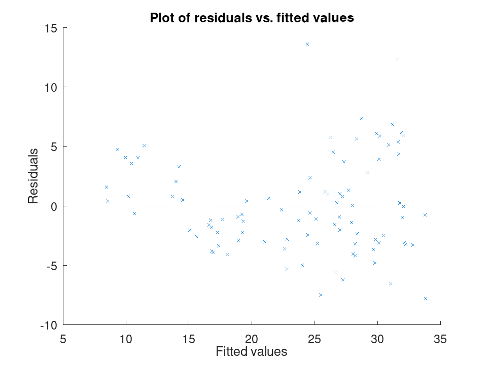
Spotting influential observations with Cook's distance. Sixteen houses are matched by size and age to a sale price, but one house was sold far above what its size and age would predict. After fitting the model, plotDiagnostics with the cookd option highlights that single observation as having outsized influence on the fit.
Size = [80; 95; 110; 120; 65; 140; 100; 130; 90; 150; 75; 105; ...
115; 85; 135; 125];
Age = [5; 10; 3; 8; 20; 2; 15; 6; 12; 1; 18; 9; 4; 14; 7; 11];
Price = [200; 230; 260; 280; 150; 320; 240; 300; 210; 340; 170; ...
250; 270; 190; 500; 290];
X = [Size, Age];
y = Price;
mdl = fitlm (X, y);
plotDiagnostics (mdl, 'cookd')
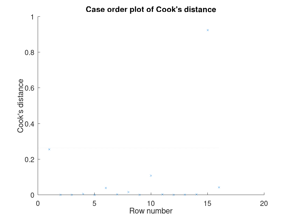
Comparing the size of each predictor's effect, alongside a hypothesis test on the model as a whole. We fit a mileage model on the carsmall data set using weight and horsepower. plotEffects draws each coefficient's estimate with its confidence interval side by side, and coefTest checks whether weight's effect is significantly different from horsepower's.
load carsmall X = [Weight, Horsepower]; y = MPG; mdl = fitlm (X, y);
Visualize the relative size of each predictor's effect.
plotEffects (mdl)
Test whether the two coefficients differ significantly.
H = [0 1 -1]; [p, F, r] = coefTest (mdl, H)
p = 0.073643 F = 3.2759 r = 1
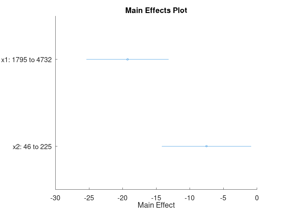
A cell array of character vectors containing the names of the predictor variables used to fit the model. This property is read-only.
Simple linear regression with a single predictor. Ten runners record their weekly training distance and their finish time in a 10k race. We fit a straight line through this data and look at the fitted coefficients, then use predict to estimate the finish time for a runner who trains a distance not in the sample.
Distance = [10; 15; 20; 25; 30; 35; 40; 45; 50; 55]; Time = [58; 55; 52; 50; 47; 45; 43; 41; 40; 38]; X = Distance; y = Time;
Fit the model and inspect the estimated slope and intercept.
mdl = fitlm (X, y)
mdl =
Linear regression model:
y ~ 1 + x1
Estimated Coefficients:
2x4 table
Estimate SE tStat pValue
________ _________ ________ ___________
(Intercept) 61.2 0.654588 93.494 1.91213e-13
x1 -0.44 0.0184226 -23.8836 1.00609e-08
Number of observations: 10, Error degrees of freedom: 8
Root Mean Squared Error: 0.83666
R-squared: 0.986169, Adjusted R-Squared: 0.984441
F-statistic vs. constant model: 570.429, p-value = 1.00609e-08
Predict the finish time for a runner training 32 km per week.
ypred = predict (mdl, 32)
ypred = 47.120
Multiple linear regression with two predictors, followed by a confidence interval on the coefficients. Thirteen coffee shops report their weekly foot traffic and the number of items on their menu, along with weekly revenue. We fit a model with both predictors, then use coefCI to see how precisely each coefficient is estimated.
Traffic = [120; 150; 90; 200; 175; 60; 220; 140; 100; 190; 80; 210; 130];
MenuSize = [8; 12; 6; 15; 10; 5; 18; 9; 7; 14; 6; 16; 11];
Revenue = [1450; 1820; 1010; 2400; 2050; 700; 2650; 1700; 1150; ...
2300; 900; 2500; 1600];
X = [Traffic, MenuSize];
y = Revenue;
Fit the model with both predictors together.
mdl = fitlm (X, y)
mdl =
Linear regression model:
y ~ 1 + x1 + x2
Estimated Coefficients:
3x4 table
Estimate SE tStat pValue
________ ________ ________ ___________
(Intercept) -47.0932 27.3456 -1.72215 0.115771
x1 11.4079 0.616078 18.517 4.55169e-09
x2 11.4344 7.68384 1.48811 0.167562
Number of observations: 13, Error degrees of freedom: 10
Root Mean Squared Error: 32.4551
R-squared: 0.997901, Adjusted R-Squared: 0.997482
F-statistic vs. constant model: 2377.53, p-value = 4.07061e-14
Check how tight the 95% confidence interval is on each coefficient.
ci = coefCI (mdl)
ci =
-108.0231 13.8366
10.0352 12.7806
-5.6862 28.5551
Growing a model with addTerms and predicting with the richer model. We model fuel economy from the carsmall data set using weight and horsepower as main effects only. addTerms then brings in the weight-horsepower interaction without needing to refit by hand, and predict shows how the estimate for a new car changes once that interaction is included.
load carsmall X = [Weight, Horsepower]; y = MPG;
Fit the additive model first.
mdl = fitlm (X, y);
Add the interaction between weight and horsepower.
mdl2 = addTerms (mdl, 'x1:x2');
Compare predictions from both models for the same new car.
Xnew = [3200, 120]; ypred1 = predict (mdl, Xnew)
ypred1 = 21.719
ypred2 = predict (mdl2, Xnew)
ypred2 = 20.416
Simplifying a model with removeTerms and comparing fit quality. We fit the full Hald cement model with all four ingredients, then use removeTerms to drop the weakest predictor and refit automatically. Comparing SSE before and after shows how little explanatory power that ingredient was actually contributing.
load hald X = ingredients; y = heat;
Fit the model with all four ingredients.
mdl = fitlm (X, y);
Drop the third ingredient and refit on the same data.
mdl2 = removeTerms (mdl, 'x3');
Compare how much the error sum of squares changed.
sse_full = mdl.SSE
sse_full = 47.864
sse_reduced = mdl2.SSE
sse_reduced = 47.973
Testing a linear hypothesis and checking residual autocorrelation. Twelve patients are given a drug at different doses over different treatment durations, and a recovery score is recorded. coefTest checks whether the dose and duration coefficients are actually equal, and dwtest separately checks whether the residuals still carry a leftover pattern the model failed to capture.
Dose = [10; 15; 20; 25; 30; 35; 12; 18; 22; 28; 32; 38]; Duration = [5; 7; 9; 11; 13; 15; 6; 8; 10; 12; 14; 16]; Recovery = [42; 48; 55; 60; 68; 74; 45; 52; 58; 65; 71; 78]; X = [Dose, Duration]; y = Recovery; mdl = fitlm (X, y);
Test H0: the Dose and Duration coefficients are equal.
H = [0 1 -1]; [p, F, r] = coefTest (mdl, H)
p = 0.3535 F = 0.9571 r = 1
Check for autocorrelation left over in the residuals.
[pdw, dw] = dwtest (mdl)
pdw = 0.3658 dw = 2.4432
Checking residuals against fitted values. We fit a mileage model on the carsmall data set using weight and horsepower, then plot the raw residuals against the fitted values. A pattern in this plot, rather than a random scatter, would suggest the linear model is missing some curvature in the relationship.
load carsmall X = [Weight, Horsepower]; y = MPG; mdl = fitlm (X, y); plotResiduals (mdl, 'fitted')
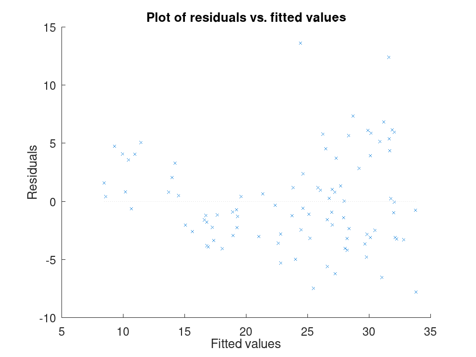
Spotting influential observations with Cook's distance. Sixteen houses are matched by size and age to a sale price, but one house was sold far above what its size and age would predict. After fitting the model, plotDiagnostics with the cookd option highlights that single observation as having outsized influence on the fit.
Size = [80; 95; 110; 120; 65; 140; 100; 130; 90; 150; 75; 105; ...
115; 85; 135; 125];
Age = [5; 10; 3; 8; 20; 2; 15; 6; 12; 1; 18; 9; 4; 14; 7; 11];
Price = [200; 230; 260; 280; 150; 320; 240; 300; 210; 340; 170; ...
250; 270; 190; 500; 290];
X = [Size, Age];
y = Price;
mdl = fitlm (X, y);
plotDiagnostics (mdl, 'cookd')
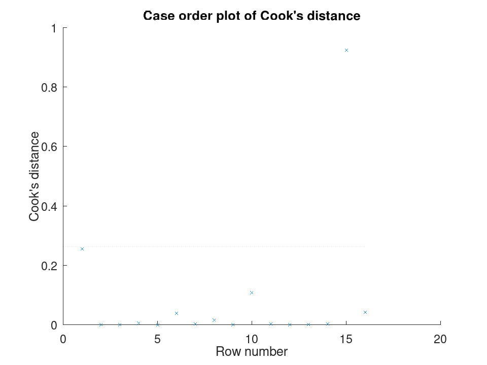
Comparing the size of each predictor's effect, alongside a hypothesis test on the model as a whole. We fit a mileage model on the carsmall data set using weight and horsepower. plotEffects draws each coefficient's estimate with its confidence interval side by side, and coefTest checks whether weight's effect is significantly different from horsepower's.
load carsmall X = [Weight, Horsepower]; y = MPG; mdl = fitlm (X, y);
Visualize the relative size of each predictor's effect.
plotEffects (mdl)
Test whether the two coefficients differ significantly.
H = [0 1 -1]; [p, F, r] = coefTest (mdl, H)
p = 0.073643 F = 3.2759 r = 1
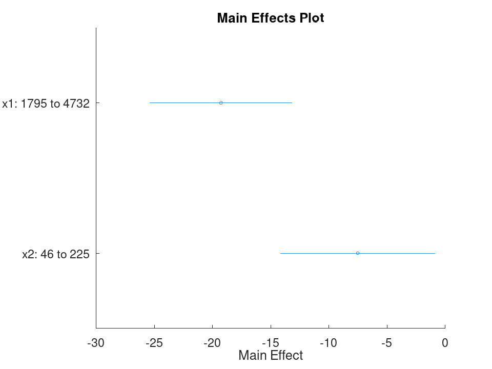
A character vector containing the name of the response variable. This property is read-only.
Simple linear regression with a single predictor. Ten runners record their weekly training distance and their finish time in a 10k race. We fit a straight line through this data and look at the fitted coefficients, then use predict to estimate the finish time for a runner who trains a distance not in the sample.
Distance = [10; 15; 20; 25; 30; 35; 40; 45; 50; 55]; Time = [58; 55; 52; 50; 47; 45; 43; 41; 40; 38]; X = Distance; y = Time;
Fit the model and inspect the estimated slope and intercept.
mdl = fitlm (X, y)
mdl =
Linear regression model:
y ~ 1 + x1
Estimated Coefficients:
2x4 table
Estimate SE tStat pValue
________ _________ ________ ___________
(Intercept) 61.2 0.654588 93.494 1.91213e-13
x1 -0.44 0.0184226 -23.8836 1.00609e-08
Number of observations: 10, Error degrees of freedom: 8
Root Mean Squared Error: 0.83666
R-squared: 0.986169, Adjusted R-Squared: 0.984441
F-statistic vs. constant model: 570.429, p-value = 1.00609e-08
Predict the finish time for a runner training 32 km per week.
ypred = predict (mdl, 32)
ypred = 47.120
Multiple linear regression with two predictors, followed by a confidence interval on the coefficients. Thirteen coffee shops report their weekly foot traffic and the number of items on their menu, along with weekly revenue. We fit a model with both predictors, then use coefCI to see how precisely each coefficient is estimated.
Traffic = [120; 150; 90; 200; 175; 60; 220; 140; 100; 190; 80; 210; 130];
MenuSize = [8; 12; 6; 15; 10; 5; 18; 9; 7; 14; 6; 16; 11];
Revenue = [1450; 1820; 1010; 2400; 2050; 700; 2650; 1700; 1150; ...
2300; 900; 2500; 1600];
X = [Traffic, MenuSize];
y = Revenue;
Fit the model with both predictors together.
mdl = fitlm (X, y)
mdl =
Linear regression model:
y ~ 1 + x1 + x2
Estimated Coefficients:
3x4 table
Estimate SE tStat pValue
________ ________ ________ ___________
(Intercept) -47.0932 27.3456 -1.72215 0.115771
x1 11.4079 0.616078 18.517 4.55169e-09
x2 11.4344 7.68384 1.48811 0.167562
Number of observations: 13, Error degrees of freedom: 10
Root Mean Squared Error: 32.4551
R-squared: 0.997901, Adjusted R-Squared: 0.997482
F-statistic vs. constant model: 2377.53, p-value = 4.07061e-14
Check how tight the 95% confidence interval is on each coefficient.
ci = coefCI (mdl)
ci =
-108.0231 13.8366
10.0352 12.7806
-5.6862 28.5551
Growing a model with addTerms and predicting with the richer model. We model fuel economy from the carsmall data set using weight and horsepower as main effects only. addTerms then brings in the weight-horsepower interaction without needing to refit by hand, and predict shows how the estimate for a new car changes once that interaction is included.
load carsmall X = [Weight, Horsepower]; y = MPG;
Fit the additive model first.
mdl = fitlm (X, y);
Add the interaction between weight and horsepower.
mdl2 = addTerms (mdl, 'x1:x2');
Compare predictions from both models for the same new car.
Xnew = [3200, 120]; ypred1 = predict (mdl, Xnew)
ypred1 = 21.719
ypred2 = predict (mdl2, Xnew)
ypred2 = 20.416
Simplifying a model with removeTerms and comparing fit quality. We fit the full Hald cement model with all four ingredients, then use removeTerms to drop the weakest predictor and refit automatically. Comparing SSE before and after shows how little explanatory power that ingredient was actually contributing.
load hald X = ingredients; y = heat;
Fit the model with all four ingredients.
mdl = fitlm (X, y);
Drop the third ingredient and refit on the same data.
mdl2 = removeTerms (mdl, 'x3');
Compare how much the error sum of squares changed.
sse_full = mdl.SSE
sse_full = 47.864
sse_reduced = mdl2.SSE
sse_reduced = 47.973
Testing a linear hypothesis and checking residual autocorrelation. Twelve patients are given a drug at different doses over different treatment durations, and a recovery score is recorded. coefTest checks whether the dose and duration coefficients are actually equal, and dwtest separately checks whether the residuals still carry a leftover pattern the model failed to capture.
Dose = [10; 15; 20; 25; 30; 35; 12; 18; 22; 28; 32; 38]; Duration = [5; 7; 9; 11; 13; 15; 6; 8; 10; 12; 14; 16]; Recovery = [42; 48; 55; 60; 68; 74; 45; 52; 58; 65; 71; 78]; X = [Dose, Duration]; y = Recovery; mdl = fitlm (X, y);
Test H0: the Dose and Duration coefficients are equal.
H = [0 1 -1]; [p, F, r] = coefTest (mdl, H)
p = 0.3535 F = 0.9571 r = 1
Check for autocorrelation left over in the residuals.
[pdw, dw] = dwtest (mdl)
pdw = 0.3658 dw = 2.4432
Checking residuals against fitted values. We fit a mileage model on the carsmall data set using weight and horsepower, then plot the raw residuals against the fitted values. A pattern in this plot, rather than a random scatter, would suggest the linear model is missing some curvature in the relationship.
load carsmall X = [Weight, Horsepower]; y = MPG; mdl = fitlm (X, y); plotResiduals (mdl, 'fitted')
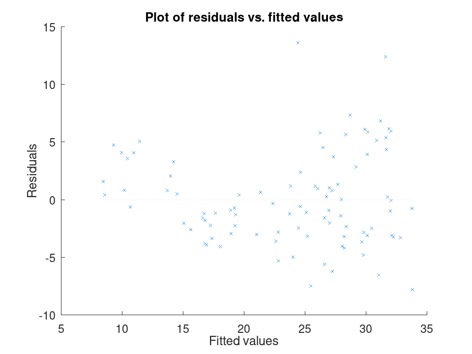
Spotting influential observations with Cook's distance. Sixteen houses are matched by size and age to a sale price, but one house was sold far above what its size and age would predict. After fitting the model, plotDiagnostics with the cookd option highlights that single observation as having outsized influence on the fit.
Size = [80; 95; 110; 120; 65; 140; 100; 130; 90; 150; 75; 105; ...
115; 85; 135; 125];
Age = [5; 10; 3; 8; 20; 2; 15; 6; 12; 1; 18; 9; 4; 14; 7; 11];
Price = [200; 230; 260; 280; 150; 320; 240; 300; 210; 340; 170; ...
250; 270; 190; 500; 290];
X = [Size, Age];
y = Price;
mdl = fitlm (X, y);
plotDiagnostics (mdl, 'cookd')
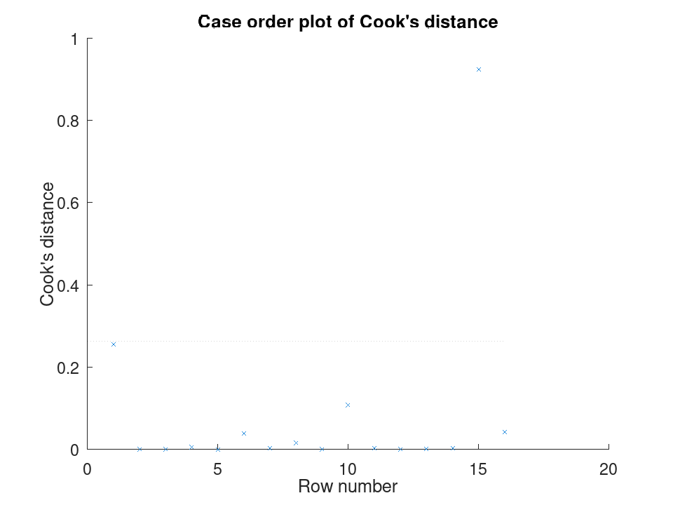
Comparing the size of each predictor's effect, alongside a hypothesis test on the model as a whole. We fit a mileage model on the carsmall data set using weight and horsepower. plotEffects draws each coefficient's estimate with its confidence interval side by side, and coefTest checks whether weight's effect is significantly different from horsepower's.
load carsmall X = [Weight, Horsepower]; y = MPG; mdl = fitlm (X, y);
Visualize the relative size of each predictor's effect.
plotEffects (mdl)
Test whether the two coefficients differ significantly.
H = [0 1 -1]; [p, F, r] = coefTest (mdl, H)
p = 0.073643 F = 3.2759 r = 1
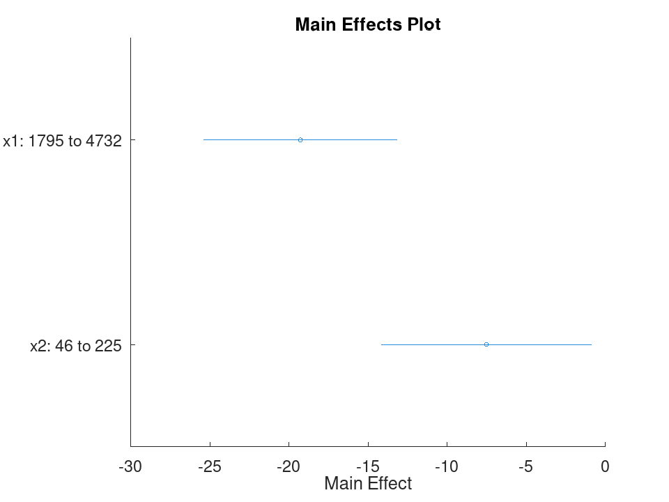
A table with one row per variable including any unused variables, and four columns:
-
Class- variable class as a character vector, e.g.'double'or'categorical' -
Range- for continuous variables, a two-element vector[min, max]; for categorical variables, a vector of the distinct values -
InModel- logical; true if the variable is in the fitted model -
IsCategorical- logical; true if the variable is categorical
This property is read-only.
Simple linear regression with a single predictor. Ten runners record their weekly training distance and their finish time in a 10k race. We fit a straight line through this data and look at the fitted coefficients, then use predict to estimate the finish time for a runner who trains a distance not in the sample.
Distance = [10; 15; 20; 25; 30; 35; 40; 45; 50; 55]; Time = [58; 55; 52; 50; 47; 45; 43; 41; 40; 38]; X = Distance; y = Time;
Fit the model and inspect the estimated slope and intercept.
mdl = fitlm (X, y)
mdl =
Linear regression model:
y ~ 1 + x1
Estimated Coefficients:
2x4 table
Estimate SE tStat pValue
________ _________ ________ ___________
(Intercept) 61.2 0.654588 93.494 1.91213e-13
x1 -0.44 0.0184226 -23.8836 1.00609e-08
Number of observations: 10, Error degrees of freedom: 8
Root Mean Squared Error: 0.83666
R-squared: 0.986169, Adjusted R-Squared: 0.984441
F-statistic vs. constant model: 570.429, p-value = 1.00609e-08
Predict the finish time for a runner training 32 km per week.
ypred = predict (mdl, 32)
ypred = 47.120
Multiple linear regression with two predictors, followed by a confidence interval on the coefficients. Thirteen coffee shops report their weekly foot traffic and the number of items on their menu, along with weekly revenue. We fit a model with both predictors, then use coefCI to see how precisely each coefficient is estimated.
Traffic = [120; 150; 90; 200; 175; 60; 220; 140; 100; 190; 80; 210; 130];
MenuSize = [8; 12; 6; 15; 10; 5; 18; 9; 7; 14; 6; 16; 11];
Revenue = [1450; 1820; 1010; 2400; 2050; 700; 2650; 1700; 1150; ...
2300; 900; 2500; 1600];
X = [Traffic, MenuSize];
y = Revenue;
Fit the model with both predictors together.
mdl = fitlm (X, y)
mdl =
Linear regression model:
y ~ 1 + x1 + x2
Estimated Coefficients:
3x4 table
Estimate SE tStat pValue
________ ________ ________ ___________
(Intercept) -47.0932 27.3456 -1.72215 0.115771
x1 11.4079 0.616078 18.517 4.55169e-09
x2 11.4344 7.68384 1.48811 0.167562
Number of observations: 13, Error degrees of freedom: 10
Root Mean Squared Error: 32.4551
R-squared: 0.997901, Adjusted R-Squared: 0.997482
F-statistic vs. constant model: 2377.53, p-value = 4.07061e-14
Check how tight the 95% confidence interval is on each coefficient.
ci = coefCI (mdl)
ci =
-108.0231 13.8366
10.0352 12.7806
-5.6862 28.5551
Growing a model with addTerms and predicting with the richer model. We model fuel economy from the carsmall data set using weight and horsepower as main effects only. addTerms then brings in the weight-horsepower interaction without needing to refit by hand, and predict shows how the estimate for a new car changes once that interaction is included.
load carsmall X = [Weight, Horsepower]; y = MPG;
Fit the additive model first.
mdl = fitlm (X, y);
Add the interaction between weight and horsepower.
mdl2 = addTerms (mdl, 'x1:x2');
Compare predictions from both models for the same new car.
Xnew = [3200, 120]; ypred1 = predict (mdl, Xnew)
ypred1 = 21.719
ypred2 = predict (mdl2, Xnew)
ypred2 = 20.416
Simplifying a model with removeTerms and comparing fit quality. We fit the full Hald cement model with all four ingredients, then use removeTerms to drop the weakest predictor and refit automatically. Comparing SSE before and after shows how little explanatory power that ingredient was actually contributing.
load hald X = ingredients; y = heat;
Fit the model with all four ingredients.
mdl = fitlm (X, y);
Drop the third ingredient and refit on the same data.
mdl2 = removeTerms (mdl, 'x3');
Compare how much the error sum of squares changed.
sse_full = mdl.SSE
sse_full = 47.864
sse_reduced = mdl2.SSE
sse_reduced = 47.973
Testing a linear hypothesis and checking residual autocorrelation. Twelve patients are given a drug at different doses over different treatment durations, and a recovery score is recorded. coefTest checks whether the dose and duration coefficients are actually equal, and dwtest separately checks whether the residuals still carry a leftover pattern the model failed to capture.
Dose = [10; 15; 20; 25; 30; 35; 12; 18; 22; 28; 32; 38]; Duration = [5; 7; 9; 11; 13; 15; 6; 8; 10; 12; 14; 16]; Recovery = [42; 48; 55; 60; 68; 74; 45; 52; 58; 65; 71; 78]; X = [Dose, Duration]; y = Recovery; mdl = fitlm (X, y);
Test H0: the Dose and Duration coefficients are equal.
H = [0 1 -1]; [p, F, r] = coefTest (mdl, H)
p = 0.3535 F = 0.9571 r = 1
Check for autocorrelation left over in the residuals.
[pdw, dw] = dwtest (mdl)
pdw = 0.3658 dw = 2.4432
Checking residuals against fitted values. We fit a mileage model on the carsmall data set using weight and horsepower, then plot the raw residuals against the fitted values. A pattern in this plot, rather than a random scatter, would suggest the linear model is missing some curvature in the relationship.
load carsmall X = [Weight, Horsepower]; y = MPG; mdl = fitlm (X, y); plotResiduals (mdl, 'fitted')
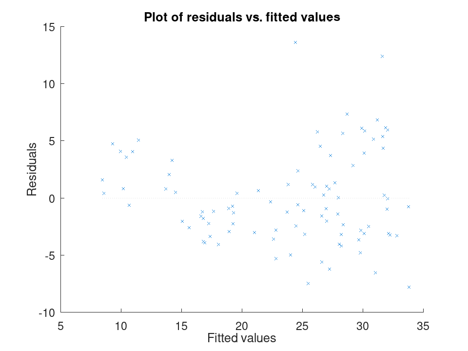
Spotting influential observations with Cook's distance. Sixteen houses are matched by size and age to a sale price, but one house was sold far above what its size and age would predict. After fitting the model, plotDiagnostics with the cookd option highlights that single observation as having outsized influence on the fit.
Size = [80; 95; 110; 120; 65; 140; 100; 130; 90; 150; 75; 105; ...
115; 85; 135; 125];
Age = [5; 10; 3; 8; 20; 2; 15; 6; 12; 1; 18; 9; 4; 14; 7; 11];
Price = [200; 230; 260; 280; 150; 320; 240; 300; 210; 340; 170; ...
250; 270; 190; 500; 290];
X = [Size, Age];
y = Price;
mdl = fitlm (X, y);
plotDiagnostics (mdl, 'cookd')
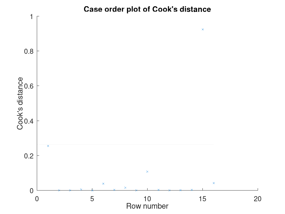
Comparing the size of each predictor's effect, alongside a hypothesis test on the model as a whole. We fit a mileage model on the carsmall data set using weight and horsepower. plotEffects draws each coefficient's estimate with its confidence interval side by side, and coefTest checks whether weight's effect is significantly different from horsepower's.
load carsmall X = [Weight, Horsepower]; y = MPG; mdl = fitlm (X, y);
Visualize the relative size of each predictor's effect.
plotEffects (mdl)
Test whether the two coefficients differ significantly.
H = [0 1 -1]; [p, F, r] = coefTest (mdl, H)
p = 0.073643 F = 3.2759 r = 1
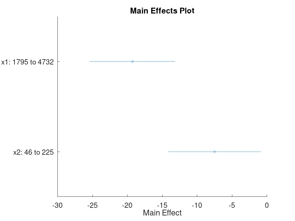
A cell array of character vectors containing the names of all
variables, including predictors, the response, and unused variables.
For table input these are the table column names. For matrix input
these are the values given by 'VarNames', defaulting to
{'x1','x2',...,'xp','y'}. This property is read-only.
Simple linear regression with a single predictor. Ten runners record their weekly training distance and their finish time in a 10k race. We fit a straight line through this data and look at the fitted coefficients, then use predict to estimate the finish time for a runner who trains a distance not in the sample.
Distance = [10; 15; 20; 25; 30; 35; 40; 45; 50; 55]; Time = [58; 55; 52; 50; 47; 45; 43; 41; 40; 38]; X = Distance; y = Time;
Fit the model and inspect the estimated slope and intercept.
mdl = fitlm (X, y)
mdl =
Linear regression model:
y ~ 1 + x1
Estimated Coefficients:
2x4 table
Estimate SE tStat pValue
________ _________ ________ ___________
(Intercept) 61.2 0.654588 93.494 1.91213e-13
x1 -0.44 0.0184226 -23.8836 1.00609e-08
Number of observations: 10, Error degrees of freedom: 8
Root Mean Squared Error: 0.83666
R-squared: 0.986169, Adjusted R-Squared: 0.984441
F-statistic vs. constant model: 570.429, p-value = 1.00609e-08
Predict the finish time for a runner training 32 km per week.
ypred = predict (mdl, 32)
ypred = 47.120
Multiple linear regression with two predictors, followed by a confidence interval on the coefficients. Thirteen coffee shops report their weekly foot traffic and the number of items on their menu, along with weekly revenue. We fit a model with both predictors, then use coefCI to see how precisely each coefficient is estimated.
Traffic = [120; 150; 90; 200; 175; 60; 220; 140; 100; 190; 80; 210; 130];
MenuSize = [8; 12; 6; 15; 10; 5; 18; 9; 7; 14; 6; 16; 11];
Revenue = [1450; 1820; 1010; 2400; 2050; 700; 2650; 1700; 1150; ...
2300; 900; 2500; 1600];
X = [Traffic, MenuSize];
y = Revenue;
Fit the model with both predictors together.
mdl = fitlm (X, y)
mdl =
Linear regression model:
y ~ 1 + x1 + x2
Estimated Coefficients:
3x4 table
Estimate SE tStat pValue
________ ________ ________ ___________
(Intercept) -47.0932 27.3456 -1.72215 0.115771
x1 11.4079 0.616078 18.517 4.55169e-09
x2 11.4344 7.68384 1.48811 0.167562
Number of observations: 13, Error degrees of freedom: 10
Root Mean Squared Error: 32.4551
R-squared: 0.997901, Adjusted R-Squared: 0.997482
F-statistic vs. constant model: 2377.53, p-value = 4.07061e-14
Check how tight the 95% confidence interval is on each coefficient.
ci = coefCI (mdl)
ci =
-108.0231 13.8366
10.0352 12.7806
-5.6862 28.5551
Growing a model with addTerms and predicting with the richer model. We model fuel economy from the carsmall data set using weight and horsepower as main effects only. addTerms then brings in the weight-horsepower interaction without needing to refit by hand, and predict shows how the estimate for a new car changes once that interaction is included.
load carsmall X = [Weight, Horsepower]; y = MPG;
Fit the additive model first.
mdl = fitlm (X, y);
Add the interaction between weight and horsepower.
mdl2 = addTerms (mdl, 'x1:x2');
Compare predictions from both models for the same new car.
Xnew = [3200, 120]; ypred1 = predict (mdl, Xnew)
ypred1 = 21.719
ypred2 = predict (mdl2, Xnew)
ypred2 = 20.416
Simplifying a model with removeTerms and comparing fit quality. We fit the full Hald cement model with all four ingredients, then use removeTerms to drop the weakest predictor and refit automatically. Comparing SSE before and after shows how little explanatory power that ingredient was actually contributing.
load hald X = ingredients; y = heat;
Fit the model with all four ingredients.
mdl = fitlm (X, y);
Drop the third ingredient and refit on the same data.
mdl2 = removeTerms (mdl, 'x3');
Compare how much the error sum of squares changed.
sse_full = mdl.SSE
sse_full = 47.864
sse_reduced = mdl2.SSE
sse_reduced = 47.973
Testing a linear hypothesis and checking residual autocorrelation. Twelve patients are given a drug at different doses over different treatment durations, and a recovery score is recorded. coefTest checks whether the dose and duration coefficients are actually equal, and dwtest separately checks whether the residuals still carry a leftover pattern the model failed to capture.
Dose = [10; 15; 20; 25; 30; 35; 12; 18; 22; 28; 32; 38]; Duration = [5; 7; 9; 11; 13; 15; 6; 8; 10; 12; 14; 16]; Recovery = [42; 48; 55; 60; 68; 74; 45; 52; 58; 65; 71; 78]; X = [Dose, Duration]; y = Recovery; mdl = fitlm (X, y);
Test H0: the Dose and Duration coefficients are equal.
H = [0 1 -1]; [p, F, r] = coefTest (mdl, H)
p = 0.3535 F = 0.9571 r = 1
Check for autocorrelation left over in the residuals.
[pdw, dw] = dwtest (mdl)
pdw = 0.3658 dw = 2.4432
Checking residuals against fitted values. We fit a mileage model on the carsmall data set using weight and horsepower, then plot the raw residuals against the fitted values. A pattern in this plot, rather than a random scatter, would suggest the linear model is missing some curvature in the relationship.
load carsmall X = [Weight, Horsepower]; y = MPG; mdl = fitlm (X, y); plotResiduals (mdl, 'fitted')
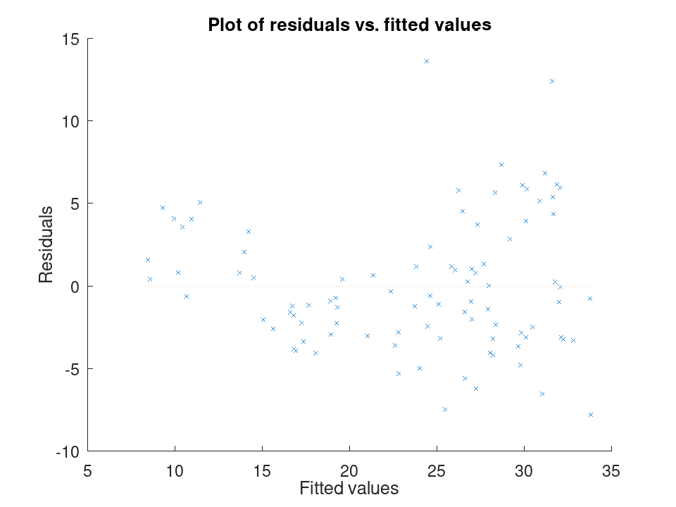
Spotting influential observations with Cook's distance. Sixteen houses are matched by size and age to a sale price, but one house was sold far above what its size and age would predict. After fitting the model, plotDiagnostics with the cookd option highlights that single observation as having outsized influence on the fit.
Size = [80; 95; 110; 120; 65; 140; 100; 130; 90; 150; 75; 105; ...
115; 85; 135; 125];
Age = [5; 10; 3; 8; 20; 2; 15; 6; 12; 1; 18; 9; 4; 14; 7; 11];
Price = [200; 230; 260; 280; 150; 320; 240; 300; 210; 340; 170; ...
250; 270; 190; 500; 290];
X = [Size, Age];
y = Price;
mdl = fitlm (X, y);
plotDiagnostics (mdl, 'cookd')
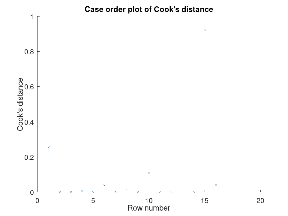
Comparing the size of each predictor's effect, alongside a hypothesis test on the model as a whole. We fit a mileage model on the carsmall data set using weight and horsepower. plotEffects draws each coefficient's estimate with its confidence interval side by side, and coefTest checks whether weight's effect is significantly different from horsepower's.
load carsmall X = [Weight, Horsepower]; y = MPG; mdl = fitlm (X, y);
Visualize the relative size of each predictor's effect.
plotEffects (mdl)
Test whether the two coefficients differ significantly.
H = [0 1 -1]; [p, F, r] = coefTest (mdl, H)
p = 0.073643 F = 3.2759 r = 1
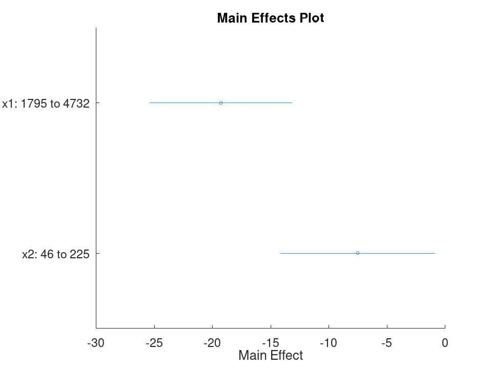
A table containing predictor and response values for all observations, including unused variables. For table input this is the full input table. For matrix input this is a table constructed from the predictor matrix and response vector. This property is read-only.
Simple linear regression with a single predictor. Ten runners record their weekly training distance and their finish time in a 10k race. We fit a straight line through this data and look at the fitted coefficients, then use predict to estimate the finish time for a runner who trains a distance not in the sample.
Distance = [10; 15; 20; 25; 30; 35; 40; 45; 50; 55]; Time = [58; 55; 52; 50; 47; 45; 43; 41; 40; 38]; X = Distance; y = Time;
Fit the model and inspect the estimated slope and intercept.
mdl = fitlm (X, y)
mdl =
Linear regression model:
y ~ 1 + x1
Estimated Coefficients:
2x4 table
Estimate SE tStat pValue
________ _________ ________ ___________
(Intercept) 61.2 0.654588 93.494 1.91213e-13
x1 -0.44 0.0184226 -23.8836 1.00609e-08
Number of observations: 10, Error degrees of freedom: 8
Root Mean Squared Error: 0.83666
R-squared: 0.986169, Adjusted R-Squared: 0.984441
F-statistic vs. constant model: 570.429, p-value = 1.00609e-08
Predict the finish time for a runner training 32 km per week.
ypred = predict (mdl, 32)
ypred = 47.120
Multiple linear regression with two predictors, followed by a confidence interval on the coefficients. Thirteen coffee shops report their weekly foot traffic and the number of items on their menu, along with weekly revenue. We fit a model with both predictors, then use coefCI to see how precisely each coefficient is estimated.
Traffic = [120; 150; 90; 200; 175; 60; 220; 140; 100; 190; 80; 210; 130];
MenuSize = [8; 12; 6; 15; 10; 5; 18; 9; 7; 14; 6; 16; 11];
Revenue = [1450; 1820; 1010; 2400; 2050; 700; 2650; 1700; 1150; ...
2300; 900; 2500; 1600];
X = [Traffic, MenuSize];
y = Revenue;
Fit the model with both predictors together.
mdl = fitlm (X, y)
mdl =
Linear regression model:
y ~ 1 + x1 + x2
Estimated Coefficients:
3x4 table
Estimate SE tStat pValue
________ ________ ________ ___________
(Intercept) -47.0932 27.3456 -1.72215 0.115771
x1 11.4079 0.616078 18.517 4.55169e-09
x2 11.4344 7.68384 1.48811 0.167562
Number of observations: 13, Error degrees of freedom: 10
Root Mean Squared Error: 32.4551
R-squared: 0.997901, Adjusted R-Squared: 0.997482
F-statistic vs. constant model: 2377.53, p-value = 4.07061e-14
Check how tight the 95% confidence interval is on each coefficient.
ci = coefCI (mdl)
ci =
-108.0231 13.8366
10.0352 12.7806
-5.6862 28.5551
Growing a model with addTerms and predicting with the richer model. We model fuel economy from the carsmall data set using weight and horsepower as main effects only. addTerms then brings in the weight-horsepower interaction without needing to refit by hand, and predict shows how the estimate for a new car changes once that interaction is included.
load carsmall X = [Weight, Horsepower]; y = MPG;
Fit the additive model first.
mdl = fitlm (X, y);
Add the interaction between weight and horsepower.
mdl2 = addTerms (mdl, 'x1:x2');
Compare predictions from both models for the same new car.
Xnew = [3200, 120]; ypred1 = predict (mdl, Xnew)
ypred1 = 21.719
ypred2 = predict (mdl2, Xnew)
ypred2 = 20.416
Simplifying a model with removeTerms and comparing fit quality. We fit the full Hald cement model with all four ingredients, then use removeTerms to drop the weakest predictor and refit automatically. Comparing SSE before and after shows how little explanatory power that ingredient was actually contributing.
load hald X = ingredients; y = heat;
Fit the model with all four ingredients.
mdl = fitlm (X, y);
Drop the third ingredient and refit on the same data.
mdl2 = removeTerms (mdl, 'x3');
Compare how much the error sum of squares changed.
sse_full = mdl.SSE
sse_full = 47.864
sse_reduced = mdl2.SSE
sse_reduced = 47.973
Testing a linear hypothesis and checking residual autocorrelation. Twelve patients are given a drug at different doses over different treatment durations, and a recovery score is recorded. coefTest checks whether the dose and duration coefficients are actually equal, and dwtest separately checks whether the residuals still carry a leftover pattern the model failed to capture.
Dose = [10; 15; 20; 25; 30; 35; 12; 18; 22; 28; 32; 38]; Duration = [5; 7; 9; 11; 13; 15; 6; 8; 10; 12; 14; 16]; Recovery = [42; 48; 55; 60; 68; 74; 45; 52; 58; 65; 71; 78]; X = [Dose, Duration]; y = Recovery; mdl = fitlm (X, y);
Test H0: the Dose and Duration coefficients are equal.
H = [0 1 -1]; [p, F, r] = coefTest (mdl, H)
p = 0.3535 F = 0.9571 r = 1
Check for autocorrelation left over in the residuals.
[pdw, dw] = dwtest (mdl)
pdw = 0.3658 dw = 2.4432
Checking residuals against fitted values. We fit a mileage model on the carsmall data set using weight and horsepower, then plot the raw residuals against the fitted values. A pattern in this plot, rather than a random scatter, would suggest the linear model is missing some curvature in the relationship.
load carsmall X = [Weight, Horsepower]; y = MPG; mdl = fitlm (X, y); plotResiduals (mdl, 'fitted')
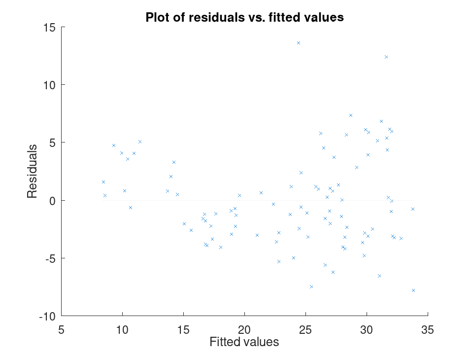
Spotting influential observations with Cook's distance. Sixteen houses are matched by size and age to a sale price, but one house was sold far above what its size and age would predict. After fitting the model, plotDiagnostics with the cookd option highlights that single observation as having outsized influence on the fit.
Size = [80; 95; 110; 120; 65; 140; 100; 130; 90; 150; 75; 105; ...
115; 85; 135; 125];
Age = [5; 10; 3; 8; 20; 2; 15; 6; 12; 1; 18; 9; 4; 14; 7; 11];
Price = [200; 230; 260; 280; 150; 320; 240; 300; 210; 340; 170; ...
250; 270; 190; 500; 290];
X = [Size, Age];
y = Price;
mdl = fitlm (X, y);
plotDiagnostics (mdl, 'cookd')
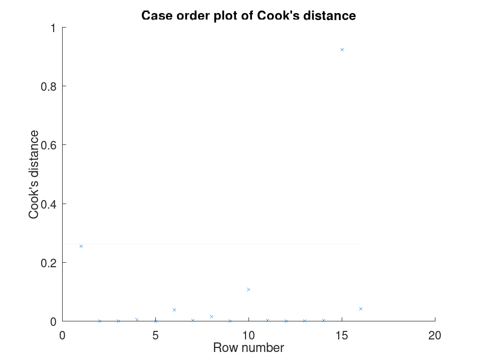
Comparing the size of each predictor's effect, alongside a hypothesis test on the model as a whole. We fit a mileage model on the carsmall data set using weight and horsepower. plotEffects draws each coefficient's estimate with its confidence interval side by side, and coefTest checks whether weight's effect is significantly different from horsepower's.
load carsmall X = [Weight, Horsepower]; y = MPG; mdl = fitlm (X, y);
Visualize the relative size of each predictor's effect.
plotEffects (mdl)
Test whether the two coefficients differ significantly.
H = [0 1 -1]; [p, F, r] = coefTest (mdl, H)
p = 0.073643 F = 3.2759 r = 1
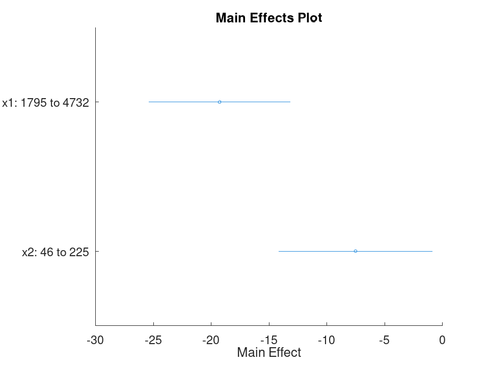
The LinearModel class offers the following public methods:
LinearModel: mdl = LinearModel (X, y)
LinearModel: mdl = LinearModel (tbl, resp_input)
LinearModel: mdl = LinearModel (…, modelspec)
LinearModel: mdl = LinearModel (…, Name, Value, …)
mdl = LinearModel (X, y) returns a
LinearModel object fit to the response y and the
predictor data X. Unless removed via the 'Intercept'
option, the fitted model contains a constant (intercept) term and one
linear term for every column of X.
-
X is an N×P numeric or logical matrix of predictor data,
where rows correspond to observations and columns correspond to
variables. By default, the predictors are named
'x1','x2', …,'xP'. -
y is an N×1 numeric or logical vector of response values,
and must have the same number of observations (rows) as X. By
default, the response is named
'y'.
mdl = LinearModel (tbl, resp_input) fits a
model using the variables in the table (or dataset) tbl as
predictors. resp_input selects the response and can be a
character vector naming a variable in tbl, or a numeric vector
the same height as tbl to use as an external response. If
resp_input is left empty, the last variable in tbl is used
as the response. Variables that are categorical arrays, cell
arrays of character vectors, or logical arrays are automatically
treated as categorical predictors.
mdl = LinearModel (…, modelspec) additionally
specifies the terms of the model to fit. modelspec can be any of
the following.
| Value | Description |
|---|---|
'constant' | Model contains only an intercept term. |
'linear' | Model contains an intercept and one term for each predictor variable. This is the default when modelspec is not specified. |
'interactions' | Model contains an intercept, all linear terms, and all pairwise products of distinct predictor variables (no squared terms). |
'purequadratic' | Model contains an intercept, all linear terms, and all squared terms. |
'quadratic' | Model contains an intercept, all linear terms, all pairwise products of distinct predictor variables, and all squared terms. |
'full' | Model contains an intercept and all terms up to and including the full P-way interaction of the predictor variables. |
| terms matrix | A T×P or T×(P+1) numeric matrix, where T is the number of terms and P is the number of predictor variables. Each row represents one term, and the value in column j is the exponent to which predictor j is raised in that term; a row of all zeros represents the intercept. If a T×(P+1) matrix is supplied, its last column (representing the response variable) must be all zeros. |
| Wilkinson formula | A character vector of the form
'y ~ terms' describing the response and predictor terms using
Wilkinson notation. For table input, the variable to the left of
'~' is used as the response, overriding resp_input. |
mdl = LinearModel (…, Name, Value,
…) specifies additional options using one or more
Name-Value pair arguments as described below.
| Name | Value |
|---|---|
'Intercept' | A logical scalar indicating
whether to include a constant (intercept) term in the model. Default
is true. Ignored when modelspec is a Wilkinson formula. |
'Weights' | A numeric vector of nonnegative observation weights, with one element per observation, used to fit a weighted least squares model. Default is a vector of ones. |
'Exclude' | A numeric or logical vector
specifying observations to exclude from the fit, given as row indices
or a logical mask. Excluded observations, together with any
observation containing a missing value, are recorded in
ObservationInfo but do not contribute to the fit. |
'CategoricalVars' | Specifies which predictor variables are treated as categorical, given as a vector of column indices, a logical vector, or a cell array of variable names. Each categorical predictor with L categories is expanded into L-1 indicator (dummy) variables, using the first category as the reference level. |
'VarNames' | A cell array of character vectors naming the predictor and response variables, in order, with the response variable name last. Only applies to matrix input, since table variables already carry their own names. |
'ResponseVar' | A character vector naming the response variable, used to override the response variable name that would otherwise be used. |
'PredictorVars' | A cell array of character vectors naming which variables in tbl to use as predictors. By default, all variables other than the response variable are used. |
'RobustOpts' | Selects ordinary least squares or
robust regression fitting. This value can be 'off' (default,
ordinary least squares), 'on' (robust fitting using the
'bisquare' weighting function), the name of one of the
weighting functions below, a function handle for a custom weighting
function, or a scalar structure with fields RobustWgtFun and
Tune specifying the weighting function and its tuning
constant. Robust fitting uses Iteratively Reweighted Least Squares
(IRLS), refitting the model with updated observation weights until the
coefficients converge. Supported weighting function names:
'andrews', 'bisquare', 'cauchy',
'fair', 'huber', 'logistic', 'ols',
'talwar', 'welsch', each with its own default tuning
constant. |
mdl is returned as a LinearModel object. If
'RobustOpts' is anything other than 'off', the returned
model is a robust fit rather than an ordinary least squares fit.
Simple linear regression with a single predictor. Ten runners record their weekly training distance and their finish time in a 10k race. We fit a straight line through this data and look at the fitted coefficients, then use predict to estimate the finish time for a runner who trains a distance not in the sample.
Distance = [10; 15; 20; 25; 30; 35; 40; 45; 50; 55]; Time = [58; 55; 52; 50; 47; 45; 43; 41; 40; 38]; X = Distance; y = Time;
Fit the model and inspect the estimated slope and intercept.
mdl = fitlm (X, y)
mdl =
Linear regression model:
y ~ 1 + x1
Estimated Coefficients:
2x4 table
Estimate SE tStat pValue
________ _________ ________ ___________
(Intercept) 61.2 0.654588 93.494 1.91213e-13
x1 -0.44 0.0184226 -23.8836 1.00609e-08
Number of observations: 10, Error degrees of freedom: 8
Root Mean Squared Error: 0.83666
R-squared: 0.986169, Adjusted R-Squared: 0.984441
F-statistic vs. constant model: 570.429, p-value = 1.00609e-08
Predict the finish time for a runner training 32 km per week.
ypred = predict (mdl, 32)
ypred = 47.120
Multiple linear regression with two predictors, followed by a confidence interval on the coefficients. Thirteen coffee shops report their weekly foot traffic and the number of items on their menu, along with weekly revenue. We fit a model with both predictors, then use coefCI to see how precisely each coefficient is estimated.
Traffic = [120; 150; 90; 200; 175; 60; 220; 140; 100; 190; 80; 210; 130];
MenuSize = [8; 12; 6; 15; 10; 5; 18; 9; 7; 14; 6; 16; 11];
Revenue = [1450; 1820; 1010; 2400; 2050; 700; 2650; 1700; 1150; ...
2300; 900; 2500; 1600];
X = [Traffic, MenuSize];
y = Revenue;
Fit the model with both predictors together.
mdl = fitlm (X, y)
mdl =
Linear regression model:
y ~ 1 + x1 + x2
Estimated Coefficients:
3x4 table
Estimate SE tStat pValue
________ ________ ________ ___________
(Intercept) -47.0932 27.3456 -1.72215 0.115771
x1 11.4079 0.616078 18.517 4.55169e-09
x2 11.4344 7.68384 1.48811 0.167562
Number of observations: 13, Error degrees of freedom: 10
Root Mean Squared Error: 32.4551
R-squared: 0.997901, Adjusted R-Squared: 0.997482
F-statistic vs. constant model: 2377.53, p-value = 4.07061e-14
Check how tight the 95% confidence interval is on each coefficient.
ci = coefCI (mdl)
ci =
-108.0231 13.8366
10.0352 12.7806
-5.6862 28.5551
Growing a model with addTerms and predicting with the richer model. We model fuel economy from the carsmall data set using weight and horsepower as main effects only. addTerms then brings in the weight-horsepower interaction without needing to refit by hand, and predict shows how the estimate for a new car changes once that interaction is included.
load carsmall X = [Weight, Horsepower]; y = MPG;
Fit the additive model first.
mdl = fitlm (X, y);
Add the interaction between weight and horsepower.
mdl2 = addTerms (mdl, 'x1:x2');
Compare predictions from both models for the same new car.
Xnew = [3200, 120]; ypred1 = predict (mdl, Xnew)
ypred1 = 21.719
ypred2 = predict (mdl2, Xnew)
ypred2 = 20.416
Simplifying a model with removeTerms and comparing fit quality. We fit the full Hald cement model with all four ingredients, then use removeTerms to drop the weakest predictor and refit automatically. Comparing SSE before and after shows how little explanatory power that ingredient was actually contributing.
load hald X = ingredients; y = heat;
Fit the model with all four ingredients.
mdl = fitlm (X, y);
Drop the third ingredient and refit on the same data.
mdl2 = removeTerms (mdl, 'x3');
Compare how much the error sum of squares changed.
sse_full = mdl.SSE
sse_full = 47.864
sse_reduced = mdl2.SSE
sse_reduced = 47.973
Testing a linear hypothesis and checking residual autocorrelation. Twelve patients are given a drug at different doses over different treatment durations, and a recovery score is recorded. coefTest checks whether the dose and duration coefficients are actually equal, and dwtest separately checks whether the residuals still carry a leftover pattern the model failed to capture.
Dose = [10; 15; 20; 25; 30; 35; 12; 18; 22; 28; 32; 38]; Duration = [5; 7; 9; 11; 13; 15; 6; 8; 10; 12; 14; 16]; Recovery = [42; 48; 55; 60; 68; 74; 45; 52; 58; 65; 71; 78]; X = [Dose, Duration]; y = Recovery; mdl = fitlm (X, y);
Test H0: the Dose and Duration coefficients are equal.
H = [0 1 -1]; [p, F, r] = coefTest (mdl, H)
p = 0.3535 F = 0.9571 r = 1
Check for autocorrelation left over in the residuals.
[pdw, dw] = dwtest (mdl)
pdw = 0.3658 dw = 2.4432
Checking residuals against fitted values. We fit a mileage model on the carsmall data set using weight and horsepower, then plot the raw residuals against the fitted values. A pattern in this plot, rather than a random scatter, would suggest the linear model is missing some curvature in the relationship.
load carsmall X = [Weight, Horsepower]; y = MPG; mdl = fitlm (X, y); plotResiduals (mdl, 'fitted')
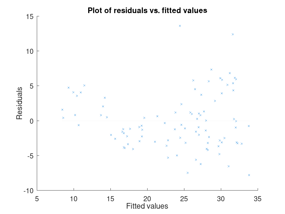
Spotting influential observations with Cook's distance. Sixteen houses are matched by size and age to a sale price, but one house was sold far above what its size and age would predict. After fitting the model, plotDiagnostics with the cookd option highlights that single observation as having outsized influence on the fit.
Size = [80; 95; 110; 120; 65; 140; 100; 130; 90; 150; 75; 105; ...
115; 85; 135; 125];
Age = [5; 10; 3; 8; 20; 2; 15; 6; 12; 1; 18; 9; 4; 14; 7; 11];
Price = [200; 230; 260; 280; 150; 320; 240; 300; 210; 340; 170; ...
250; 270; 190; 500; 290];
X = [Size, Age];
y = Price;
mdl = fitlm (X, y);
plotDiagnostics (mdl, 'cookd')
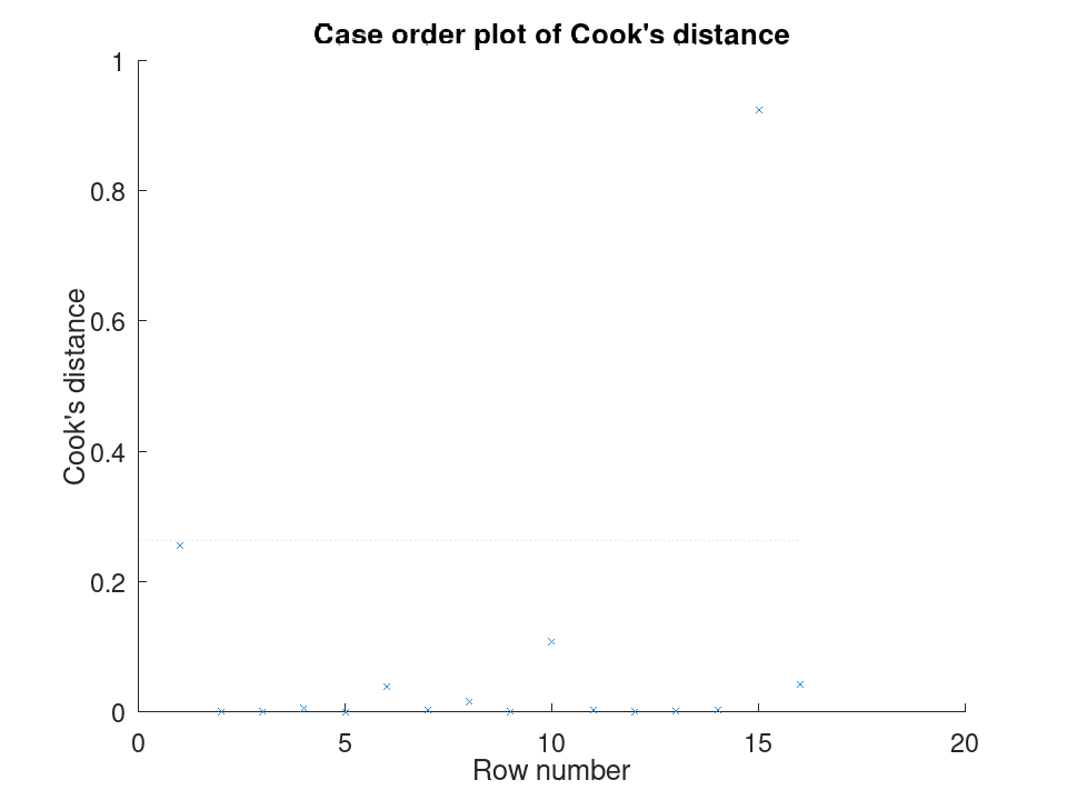
Comparing the size of each predictor's effect, alongside a hypothesis test on the model as a whole. We fit a mileage model on the carsmall data set using weight and horsepower. plotEffects draws each coefficient's estimate with its confidence interval side by side, and coefTest checks whether weight's effect is significantly different from horsepower's.
load carsmall X = [Weight, Horsepower]; y = MPG; mdl = fitlm (X, y);
Visualize the relative size of each predictor's effect.
plotEffects (mdl)
Test whether the two coefficients differ significantly.
H = [0 1 -1]; [p, F, r] = coefTest (mdl, H)
p = 0.073643 F = 3.2759 r = 1
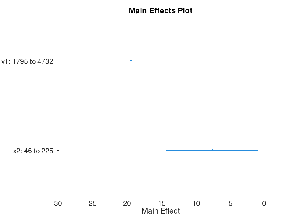
LinearModel: ypred = predict (mdl, Xnew)
LinearModel: ypred = predict (mdl)
LinearModel: [ypred, yci] = predict (mdl, Xnew)
LinearModel: [ypred, yci] = predict (mdl, Xnew, Name, Value)
ypred = predict (mdl, Xnew) returns the fitted
response values at the new predictor locations in Xnew. Xnew
can be a numeric matrix with one column per predictor in the same order
as the training data, or a table whose column names match
mdl.PredictorNames. Rows containing NaN are returned
as NaN without error.
ypred = predict (mdl) omits Xnew and returns
fitted values for the original training observations in their original
row order. Rows that were excluded or contained missing values are
returned as NaN. The result is identical to
mdl.Fitted.
[ypred, yci] = predict (…) also returns
yci, an n-by-2 matrix of confidence bounds where column 1 is
the lower bound and column 2 is the upper bound. By default these are
95% pointwise confidence intervals on the mean response.
Name-Value pair arguments:
| Name | Value |
|---|---|
'Alpha' | Significance level for the confidence
interval, specified as a scalar in [0,1]. The interval has
coverage 100(1-\alpha)\%. Default is 0.05, giving a 95%
interval. |
'Prediction' | Type of interval to compute.
"curve" (default) gives a confidence interval on the mean response
f(x). "observation" gives a wider prediction interval for
a single future observation y = f(x) + \varepsilon, which accounts
for both estimation uncertainty and irreducible noise; it adds
mdl.MSE to the variance before computing the half-width. |
'Simultaneous' | Logical flag controlling whether
the bounds are simultaneous or pointwise. When true,
Scheff'{e}’s method is used so the entire predicted curve lies within
the band with 100(1-\alpha)\% confidence; these bands are always
wider than pointwise ones. Default is false. |
Predicting with and without new data. Ten students study for varying numbers of hours before an exam, with their resulting scores recorded. Calling predict with no Xnew returns the fitted values for the training data itself (the same as mdl.Fitted); calling it with new hour values predicts scores at points not in the original sample, including one beyond the range of the data.
Hours = [1;2;3;4;5;6;7;8;9;10]; Score = [52;55;61;64;70;73;77;81;85;90]; mdl = fitlm (Hours, Score);
Fitted values for the original training data.
fitted = predict (mdl)
fitted = 51.873 56.079 60.285 64.491 68.697 72.903 77.109 81.315 85.521 89.727
Predictions at 5.5 hours (interpolation) and 11 hours (extrapolation).
ypred = predict (mdl, [5.5; 11])
ypred = 70.800 93.933
Confidence intervals versus prediction intervals, and simultaneous bounds. Twelve students' exam scores depend on both study hours and hours of sleep. The default output is a 95% confidence interval on the mean response; 'Prediction', 'observation' widens it to account for a single future observation instead of the average; and 'Simultaneous', true widens it further so the whole predicted surface, not just each point individually, holds at the stated confidence level.
Hours = [1;2;3;4;5;6;7;8;9;10;11;12]; Sleep = [5;6;5;7;6;8;7;6;8;7;9;8]; Score = [50;54;56;62;64;70;71;73;79;78;85;84]; X = [Hours, Sleep]; mdl = fitlm (X, Score); Xnew = [6 7; 10 8];
Default: 95% confidence interval on the mean response.
[ypred, yci_curve] = predict (mdl, Xnew)
ypred = 67.751 80.461 yci_curve = 66.977 68.525 79.426 81.495
Wider prediction interval for a single new observation.
[ypred, yci_obs] = predict (mdl, Xnew, 'Prediction', 'observation')
ypred = 67.751 80.461 yci_obs = 65.163 70.340 77.782 83.139
90% simultaneous confidence band over both points at once.
[ypred, yci_sim] = predict (mdl, Xnew, 'Alpha', 0.1, 'Simultaneous', true)
ypred = 67.751 80.461 yci_sim = 66.758 68.745 79.132 81.789
Predicting fuel economy from a quadratic model of vehicle weight, using the carsmall data set. fitlm fits MPG as a quadratic function of Weight, and predict computes the fitted curve at every original weight value, showing how well the quadratic term captures the curvature that a straight line would miss.
load carsmall X = Weight; y = MPG; mdl = fitlm (X, y, 'quadratic');
Predicted fuel economy for the first five cars in the data set.
ypred = predict (mdl, X); ypred(1:5)
ans = 18.490 17.038 19.030 19.054 18.926
Predicting from a CompactLinearModel gives the same answer as the original model, at a fraction of the memory footprint. Eight months of advertising spend and sales are used to fit a simple model. compact discards the training data but keeps everything predict needs; unlike LinearModel, Xnew cannot be omitted here, since a compact model has no training data to fall back on.
AdSpend = [10;20;30;40;50;60;70;80]; Sales = [15;18;24;27;33;36;42;45]; mdl = fitlm (AdSpend, Sales); cmdl = compact (mdl); Xnew = [25; 55];
Predictions from the full model.
[ypred_full, yci_full] = predict (mdl, Xnew)
ypred_full = 21.143 34.429 yci_full = 20.172 22.113 33.631 35.226
Predictions from the compact model match exactly.
[ypred_compact, yci_compact] = predict (cmdl, Xnew)
ypred_compact = 21.143 34.429 yci_compact = 20.172 22.113 33.631 35.226
LinearModel: ysim = random (mdl, Xnew)
ysim = random (mdl, Xnew) computes the fitted
response at each row of Xnew and then adds independent Gaussian
noise to each value. The noise is drawn from N(0, \sigma^2) where
\sigma^2 is the estimated error variance mdl.MSE
(mean squared error of the fit). The result is a column vector of the
same length as the number of rows in Xnew.
Xnew is required and must be non-empty. It can be a numeric
matrix with one column per predictor in the same order as the training
data, or a table whose column names match
mdl.PredictorNames. Unlike predict, there is no
no-argument form; the predictor locations must always be supplied
explicitly.
Because the added noise is drawn freshly on every call, two calls with
the same Xnew will generally produce different output. To get
reproducible results, set the random seed with rand ('state', s)
before calling random.
For deterministic predictions without noise, use predict or
feval. predict also provides confidence intervals on the
mean response.
Simulating noisy responses versus the deterministic fitted value. Seven days' temperatures and ice-cream sales are used to fit a simple model. predict gives the deterministic fitted value at each new temperature; random adds independent Gaussian noise scaled by the model's mean squared error, giving a plausible simulated observation instead.
Temp = [60;65;70;75;80;85;90]; Sales = [200;230;260;300;340;370;410]; mdl = fitlm (Temp, Sales); Xnew = [72; 88];
The deterministic fitted value, with no noise.
ypred = predict (mdl, Xnew)
ypred = 280.21 393.36
A simulated observation at the same points, with noise added.
ysim = random (mdl, Xnew)
ysim = 282.02 404.38
Reproducible simulated responses by seeding the generator that random actually draws from. random adds its noise with randn, so reproducibility comes from seeding randn itself, not rand. Resetting to the same state before each call gives back the exact same simulated values.
rng (42);
randg ('state', 42);
Temp = [60;65;70;75;80;85;90];
Sales = [200;230;260;300;340;370;410];
mdl = fitlm (Temp, Sales);
Xnew = [72; 88];
Two calls from the same seed give identical simulated responses.
ysimA = random (mdl, Xnew); ysimB = random (mdl, Xnew); same_seed_matches = isequal (ysimA, ysimB)
same_seed_matches = 0
Simulating noisy fuel-economy readings from a quadratic model of vehicle weight, using the carsmall data set. The deterministic quadratic fit gives a smooth predicted curve; random adds noise scaled by the model's own MSE to produce plausible individual readings a new car of that weight might show.
rng (42);
randg ('state', 42);
load carsmall
X = Weight;
y = MPG;
mdl = fitlm (X, y, 'quadratic');
Xsub = X(1:5);
Deterministic predictions for the first five cars.
ypred = predict (mdl, Xsub)
ypred = 18.490 17.038 19.030 19.054 18.926
Simulated readings for the same five cars, with noise added.
ysim = random (mdl, Xsub)
ysim = 18.463 15.073 16.096 24.235 14.062
random on a CompactLinearModel gives the same simulated draw as the original model, given the same seed. compact discards the training data but keeps everything random needs; reseeding identically before each call confirms the compact model simulates exactly the same values as the original.
rng (42);
randg ('state', 42);
Temp = [60;65;70;75;80;85;90];
Sales = [200;230;260;300;340;370;410];
mdl = fitlm (Temp, Sales);
cmdl = compact (mdl);
Xnew = [72; 88];
Same seed, same simulated draw from either model.
ysim_full = random (mdl, Xnew); ysim_compact = random (cmdl, Xnew); compact_matches_full = isequal (ysim_full, ysim_compact)
compact_matches_full = 0
LinearModel: ypred = feval (mdl, X)
LinearModel: ypred = feval (mdl, x1, x2, …, xp)
ypred = feval (mdl, X) accepts a single
numeric matrix X with one column per predictor in the same order
as the training data, or a table whose column names match
mdl.PredictorNames. The output is an n-by-1 column
vector. Rows that contain NaN in any predictor column are
returned as NaN.
ypred = feval (mdl, x1, x2, …,
xp) accepts exactly mdl.NumPredictors separate
arguments, one per predictor variable. All non-scalar arguments must
have the same size; a scalar argument is broadcast to that size
automatically. The output shape follows the shape of the non-scalar
inputs: column vector inputs give a column vector output, row vector
inputs give a row vector output, and all-scalar inputs give a scalar.
This form is convenient when predictor data is already stored in separate
vectors rather than a combined matrix.
feval gives the same numerical predictions as predict but
does not support confidence intervals. Use predict when you also
need bounds on the response. Because a LinearModel object behaves
like a function through feval, it can be passed directly to
routines that accept a function handle, such as fminsearch or
integral.
The matrix form, the separate-argument form, and broadcasting a scalar against a vector. Ten students' exam scores depend on both study hours and hours of sleep. feval accepts predictors either as one matrix, one column per predictor, or as separate arguments in the same order; a scalar argument is broadcast against any non-scalar ones, so a single sleep value can be paired with several study-hour values at once.
Hours = [1;2;3;4;5;6;7;8;9;10]; Sleep = [5;6;5;7;6;8;7;6;8;7]; Score = [50;54;56;62;64;70;71;73;79;78]; mdl = fitlm ([Hours, Sleep], Score);
Predictor data as a single matrix, one column per predictor.
ypred_matrix = feval (mdl, [6 7; 10 8])
ypred_matrix = 68.006 81.311
The same points, as separate arguments instead.
ypred_sep = feval (mdl, [6;10], [7;8])
ypred_sep = 68.006 81.311
Three study-hour values, all paired with the same 7 hours of sleep.
ypred_broadcast = feval (mdl, [4;6;8], 7)
ypred_broadcast = 62.209 68.006 73.802
Passing a categorical predictor's level directly as a plain string, no table required. Nine stores in three regions report ad spend and sales. In the separate-argument form, a categorical predictor's value can be given as its level name directly, giving the same answer as building a one-row table by hand.
AdSpend = [10;20;30;15;25;35;12;22;32];
Region = {'North';'North';'North';'South';'South';'South'; ...
'East';'East';'East'};
Sales = [15;18;24;20;27;33;12;19;26];
T = table (AdSpend, Region, Sales);
mdl = fitlm (T, 'Sales ~ AdSpend + Region', 'CategoricalVars', {'Region'});
A one-row table with AdSpend 20 and Region 'South'.
ypred_table = feval (mdl, table (20, {'South'}, ...
'VariableNames', {'AdSpend','Region'}))
ypred_table = 23.667
The same prediction, passing the level name directly.
ypred_sep = feval (mdl, 20, 'South')
ypred_sep = 23.667
A fitted model behaves like an ordinary function handle, so it can be passed straight into routines such as fminsearch. A quadratic model of fuel economy against vehicle weight is fit on the carsmall data set. Wrapping feval in an anonymous function lets fminsearch search for the weight at which the model predicts exactly 25 MPG, without ever calling predict directly.
load carsmall X = Weight; y = MPG; mdl = fitlm (X, y, 'quadratic'); target = 25;
Search for the weight giving a predicted fuel economy of 25 MPG.
wopt = fminsearch (@(w) (feval (mdl, w) - target)^2, 3000)
wopt = 2752.4
Confirm the prediction at that weight.
mpg_at_wopt = feval (mdl, wopt)
mpg_at_wopt = 25.000
feval on a CompactLinearModel gives identical results to the original model, in both calling forms. Reusing the study-hours-and-sleep model, compact discards the training data but keeps everything feval needs, so both the matrix form and the separate-argument form still work exactly as before.
Hours = [1;2;3;4;5;6;7;8;9;10]; Sleep = [5;6;5;7;6;8;7;6;8;7]; Score = [50;54;56;62;64;70;71;73;79;78]; mdl = fitlm ([Hours, Sleep], Score); cmdl = compact (mdl);
Matrix form: full model versus compact model.
ypred_full = feval (mdl, [6 7; 10 8])
ypred_full = 68.006 81.311
ypred_compact = feval (cmdl, [6 7; 10 8])
ypred_compact = 68.006 81.311
Separate-argument form: full model versus compact model.
ypred_full_sep = feval (mdl, [6;10], [7;8])
ypred_full_sep = 68.006 81.311
ypred_compact_sep = feval (cmdl, [6;10], [7;8])
ypred_compact_sep = 68.006 81.311
LinearModel: ci = coefCI (mdl)
LinearModel: ci = coefCI (mdl, alpha)
ci = coefCI (mdl) returns 95% confidence intervals
for every coefficient in mdl using a default significance level of
0.05.
ci = coefCI (mdl, alpha) uses the significance
level alpha, a scalar in [0, 1]. The resulting intervals
have coverage 100(1-\alpha)\%. Setting alpha to 0
produces intervals of infinite width; setting it to 1 collapses
each interval to the corresponding point estimate.
The output ci is a k-by-2 numeric matrix where
k = mdl.NumCoefficients. Row j contains
the interval for the j-th coefficient, whose name is stored in
mdl.CoefficientNames{j}. Column 1 is the lower bound and
column 2 is the upper bound. The midpoint of each interval equals the
corresponding point estimate in mdl.Coefficients.Estimate.
Intervals use the Wald method:
b_j \pm t_{(1-\alpha/2,\,\mathrm{DFE})}\,\mathrm{SE}(b_j),
where b_j is the coefficient estimate, \mathrm{SE}(b_j) is
its standard error from mdl.Coefficients.SE, and the
critical value is the 1-\alpha/2 quantile of the
t-distribution with mdl.DFE degrees of freedom.
In rank-deficient models, aliased coefficients have
\mathrm{SE} = 0 and their row in ci is [0, 0].
Default 95% confidence intervals versus a custom significance level. Ten students' exam scores are modeled against study hours. The default call gives 95% intervals; passing alpha explicitly gives intervals of a different width, always centered on the same point estimate.
Hours = [1;2;3;4;5;6;7;8;9;10]; Score = [52;55;61;64;70;73;77;81;85;90]; mdl = fitlm (Hours, Score);
Default 95% confidence intervals.
ci95 = coefCI (mdl)
ci95 =
46.5393 48.7940
4.0244 4.3877
Narrower 90% intervals, using alpha = 0.10.
ci90 = coefCI (mdl, 0.10)
ci90 =
46.7576 48.5757
4.0596 4.3526
A rank-deficient model: an aliased coefficient's interval collapses to [0, 0]. x2 is defined as exactly twice x1, so the design matrix is rank deficient and the two predictors cannot be told apart. The model keeps x1 and aliases x2, whose standard error is zero and whose confidence interval is reported as [0, 0] rather than a meaningless point estimate with no uncertainty.
x1 = [1;2;3;4;5;6;7;8]; x2 = 2*x1; y = 3 + 1.5*x1 + 0.5*sin ((1:8)'); mdl = fitlm ([x1, x2], y);
The second row, for x2, is exactly [0, 0].
ci = coefCI (mdl)
ci =
2.3421 3.9413
0 0
0.6658 0.8241
Confidence intervals for a four-predictor model, at two confidence levels, using the hald cement data set. Four chemical percentages in cement (ingredients) are used to predict heat given off while hardening (heat). With only 13 observations and four predictors, several intervals are wide enough to include zero.
load hald mdl = fitlm (ingredients, heat);
95% confidence intervals for all four coefficients.
ci_95 = coefCI (mdl)
ci_95 =
-99.1786 223.9893
-0.1663 3.2685
-1.1589 2.1792
-1.6385 1.8423
-1.7791 1.4910
Narrower 90% confidence intervals for comparison.
ci_90 = coefCI (mdl, 0.10)
ci_90 =
-67.8949 192.7057
0.1662 2.9360
-0.8358 1.8561
-1.3015 1.5053
-1.4626 1.1745
coefCI on a CompactLinearModel gives the same intervals as the original model. compact discards the training data but keeps everything coefCI needs: the coefficient estimates, their standard errors, and the error degrees of freedom.
Hours = [1;2;3;4;5;6;7;8;9;10]; Score = [52;55;61;64;70;73;77;81;85;90]; mdl = fitlm (Hours, Score); cmdl = compact (mdl);
Confidence intervals from the full model.
ci_full = coefCI (mdl)
ci_full =
46.5393 48.7940
4.0244 4.3877
Confidence intervals from the compact model match exactly.
ci_compact = coefCI (cmdl)
ci_compact =
46.5393 48.7940
4.0244 4.3877
LinearModel: p = coefTest (mdl)
LinearModel: p = coefTest (mdl, H)
LinearModel: p = coefTest (mdl, H, C)
LinearModel: [p, F] = coefTest (…)
LinearModel: [p, F, r] = coefTest (…)
coefTest tests whether one or more linear combinations of the
fitted coefficients equal specified constants. Each linear combination
is encoded as a row of the contrast matrix H, and the right-hand
side is given by C.
p = coefTest (mdl) performs the overall model F-test:
it tests the joint null hypothesis that every coefficient except the
intercept is zero. The returned p-value matches the F-statistic line
printed at the bottom of the model display.
p = coefTest (mdl, H) tests the null hypothesis
H \beta = 0, where \beta is the full coefficient vector
of length k = mdl.NumCoefficients. H must be
a full-rank numeric matrix with k columns; each row specifies one
linear constraint. To test a single coefficient, use a row vector with a
1 in that coefficient’s position and zeros elsewhere; the
resulting F-statistic equals the square of the corresponding t-statistic
in mdl.Coefficients. To test a categorical predictor that
expands to multiple indicator columns, include one row per indicator in
H.
p = coefTest (mdl, H, C) tests
H \beta = C instead of zero. C must be a numeric vector
with the same number of elements as rows of H; both row and column
vectors are accepted.
The second output F is the value of the F-statistic:
F = (H\hat{\beta} - C)^\prime (H V H^\prime)^{-1}
(H\hat{\beta} - C) / r, where V is
mdl.CoefficientCovariance and r is the number of
rows of H. The third output r is that numerator degrees of
freedom; the denominator degrees of freedom is mdl.DFE.
Under the null hypothesis F follows an F(r, \mathrm{DFE})
distribution and the p-value is the upper-tail probability. When
H is rank-deficient but contains no NaN, both p and
F are returned as NaN without an error.
The overall model F-test, with no H supplied. Ten students' exam scores are modeled against study hours. coefTest with no arguments tests the joint null hypothesis that every coefficient except the intercept is zero -- the same test summarized in the "F-statistic vs. constant model" line at the bottom of the model display.
Hours = [1;2;3;4;5;6;7;8;9;10]; Score = [52;55;61;64;70;73;77;81;85;90]; mdl = fitlm (Hours, Score);
The overall F-test: p-value, F-statistic, and numerator DF.
[p, F, r] = coefTest (mdl)
p = 1.6808e-11 F = 2849.9 r = 1
Compare against the F-statistic line printed for the model itself.
mdl
mdl =
Linear regression model:
y ~ 1 + x1
Estimated Coefficients:
2x4 table
Estimate SE tStat pValue
________ _________ _______ ___________
(Intercept) 47.6667 0.488866 97.5046 1.36679e-13
x1 4.20606 0.0787879 53.3846 1.68076e-11
Number of observations: 10, Error degrees of freedom: 8
Root Mean Squared Error: 0.715626
R-squared: 0.997201, Adjusted R-Squared: 0.996851
F-statistic vs. constant model: 2849.92, p-value = 1.68076e-11
Jointly testing every indicator column of a categorical predictor at once. Nine stores in three regions report ad spend and sales. Region expands to two indicator coefficients, Region_South and Region_East; a two-row H, one row per indicator, tests whether both are zero together -- whether region has any effect on sales at all, as a single joint test rather than two separate ones.
AdSpend = [10;20;30;15;25;35;12;22;32];
Region = {'North';'North';'North';'South';'South';'South'; ...
'East';'East';'East'};
Sales = [15;18;24;20;27;33;12;19;26];
T = table (AdSpend, Region, Sales);
mdl = fitlm (T, 'Sales ~ AdSpend + Region', 'CategoricalVars', {'Region'});
Coefficient order: (Intercept), AdSpend, Region_South, Region_East.
mdl.CoefficientNames
ans =
1x4 cell array
{'(Intercept)'} {'AdSpend'} {'Region_South'} {'Region_East'}
Joint test that both region coefficients are zero.
[p, F, r] = coefTest (mdl, [0 0 1 0; 0 0 0 1])
p = 6.7547e-03 F = 15.954 r = 2
Testing a coefficient against a specific hypothesized value, not just zero, using the H, C form. Four chemical percentages in cement (ingredients) are used to predict heat given off while hardening (heat), using the hald data set. Rather than testing whether the coefficient for x1 is zero, H picks out that coefficient and C supplies the hypothesized value 1.5 to test it against instead.
load hald mdl = fitlm (ingredients, heat);
Coefficient order: (Intercept), x1, x2, x3, x4.
mdl.CoefficientNames
ans =
1x5 cell array
{'(Intercept)'} {'x1'} {'x2'} {'x3'} {'x4'}
Test whether the coefficient for x1 equals 1.5.
[p, F, r] = coefTest (mdl, [0 1 0 0 0], 1.5)
p = 0.9470 F = 4.7081e-03 r = 1
coefTest on a CompactLinearModel gives the same results as the original model, for both the overall test and a specific H. compact discards the training data but keeps everything coefTest needs: the coefficient estimates, their covariance, and the error degrees of freedom.
Hours = [1;2;3;4;5;6;7;8;9;10]; Score = [52;55;61;64;70;73;77;81;85;90]; mdl = fitlm (Hours, Score); cmdl = compact (mdl);
The overall F-test matches exactly.
[p_full, F_full, r_full] = coefTest (mdl)
p_full = 1.6808e-11 F_full = 2849.9 r_full = 1
[p_compact, F_compact, r_compact] = coefTest (cmdl)
p_compact = 1.6808e-11 F_compact = 2849.9 r_compact = 1
A specific single-coefficient test also matches exactly.
[p_full2, F_full2] = coefTest (mdl, [0 1])
p_full2 = 1.6808e-11 F_full2 = 2849.9
[p_compact2, F_compact2] = coefTest (cmdl, [0 1])
p_compact2 = 1.6808e-11 F_compact2 = 2849.9
LinearModel: p = dwtest (mdl)
LinearModel: p = dwtest (mdl, method)
LinearModel: p = dwtest (mdl, method, tail)
LinearModel: [p, DW] = dwtest (…)
dwtest checks whether the raw residuals of mdl are
correlated with their immediate neighbours in observation order, which
would violate the independence assumption of ordinary least squares.
The null hypothesis is that there is no autocorrelation. A small
p-value gives evidence against this and suggests that the residuals are
not independent. This test is most meaningful when the observations
have a natural ordering, such as a time series.
The test is based on the Durbin-Watson statistic DW = \sum_{i=1}^{n-1}(e_{i+1}-e_i)^2 / \sum_{i=1}^{n}e_i^2, where e_i are the raw residuals of the active (non-excluded) observations. The statistic always lies in [0, 4]: values near 2 indicate no autocorrelation, values well below 2 indicate positive autocorrelation (adjacent residuals tend to have the same sign), and values well above 2 indicate negative autocorrelation (adjacent residuals tend to alternate in sign).
method controls how the p-value is computed and defaults to
'exact'. 'exact' uses the eigenvalues of the
projected differencing matrix together with Imhof’s numerical
integration to obtain a precise p-value; this is slower but accurate
for any sample size. 'approximate' uses a normal approximation
based on the first two moments of the DW distribution under the null;
this is faster and adequate for large samples but less reliable for
small ones. The argument is case-insensitive.
tail selects the alternative hypothesis and defaults to
'both'. 'right' tests for positive autocorrelation
(DW < 2), 'left' tests for negative autocorrelation
(DW > 2), and 'both' tests for autocorrelation in
either direction. The one-sided p-values always satisfy
p_{\mathrm{right}} + p_{\mathrm{left}} = 1, and the two-sided
p-value equals 2\min(p_{\mathrm{right}}, p_{\mathrm{left}}).
The second output DW is the value of the Durbin-Watson statistic itself; it does not depend on method or tail.
Basic usage: the Durbin-Watson statistic and its p-value. Fifteen measurements are taken over time, with a small oscillation layered on top of an otherwise linear trend. The DW statistic comes out close to but above 2, and the default two-sided p-value gives no strong evidence of autocorrelation at the usual 0.05 threshold.
Time = (1:15)'; Value = 10 + 0.5*Time + 0.4*sin (Time*2.1); mdl = fitlm (Time, Value);
The p-value and the DW statistic itself.
[p, DW] = dwtest (mdl)
p = 0.092537 DW = 2.9384
Comparing the 'exact' and 'approximate' methods, and confirming the one-sided tails sum to 1. The DW statistic itself never depends on method; only the p-value computation changes. The right-tailed and left-tailed p-values always add up to exactly 1, and the two-sided p-value equals twice the smaller of the two.
Time = (1:15)'; Value = 10 + 0.5*Time + 0.4*sin (Time*2.1); mdl = fitlm (Time, Value);
The exact and normal-approximation methods give close but distinct p-values, for the same DW statistic.
[p_exact, DW] = dwtest (mdl, 'exact')
p_exact = 0.092537 DW = 2.9384
[p_approx, DW] = dwtest (mdl, 'approximate')
p_approx = 0.096182 DW = 2.9384
The two one-sided tails always sum to 1.
p_right = dwtest (mdl, 'exact', 'right')
p_right = 0.9537
p_left = dwtest (mdl, 'exact', 'left')
p_left = 0.046269
sum_tails = p_right + p_left
sum_tails = 1
Detecting autocorrelation introduced by the natural row order of a real data set. Fitting fuel economy against weight in the carsmall data set gives a DW statistic well below 2 and a tiny p-value, since cars from the same manufacturer or model year tend to sit near each other in the table and share similar residuals -- autocorrelation can show up from any meaningful row ordering, not only from a time series.
load carsmall mdl = fitlm (Weight, MPG);
A DW statistic well below 2, with a highly significant p-value.
[p, DW] = dwtest (mdl)
p = 8.0185e-07 DW = 1.0593
Distinguishing positive from negative autocorrelation. Two series share the same linear trend but oscillate at different speeds. The fast oscillation makes neighbouring residuals swing to opposite signs, which dwtest reports as negative autocorrelation (DW pushed above 2); the slow oscillation makes neighbouring residuals stay similar for long stretches, which reads as positive autocorrelation instead (DW pushed toward 0). Both are strongly significant, just in opposite directions.
x = (1:20)';
Fast oscillation: negative autocorrelation (DW above 2).
y_fast = 5 + 2*x + 3*sin (x*2.3); mdl_fast = fitlm (x, y_fast); [p_fast, DW_fast] = dwtest (mdl_fast)
p_fast = 0.010044 DW_fast = 3.1309
Slow oscillation: positive autocorrelation (DW near 0).
y_slow = 5 + 2*x + 4*sin (x*0.3); mdl_slow = fitlm (x, y_slow); [p_slow, DW_slow] = dwtest (mdl_slow)
p_slow = 2.5959e-09 DW_slow = 0.2633
LinearModel: NewMdl = addTerms (mdl, terms)
addTerms returns a new LinearModel refitted on the same
data and settings as mdl with the specified terms appended
to the model formula. The original model mdl is never modified;
all settings including observation weights, excluded rows, and
categorical variable encodings are carried over automatically. To
update a model in place, reassign the result:
mdl = addTerms (mdl, terms).
terms may be a character vector in Wilkinson notation. Use
'x1' for a main effect, 'x1:x2' for a two-way
interaction, 'x1*x2' to add both main effects and their
interaction in one step, 'x1 + x2^2' to add several terms at
once, or '1' to add an intercept to a no-intercept model. A
bare power term 'x1^2' adds x1 together with
x1^2 (and any intermediate powers), matching the Wilkinson
hierarchy convention; power notation used inside an interaction, e.g.
'x1:x2^2', adds only that exact interaction term. All
variable names must match entries in mdl.PredictorNames.
terms may also be a numeric matrix of size t-by-v,
where t is the number of terms to add and v equals
mdl.NumVariables. Entry T(i,j) is the exponent of
variable j in term i. For example, in a model with
variables x1, x2, y: [0 0 0] is the
intercept, [0 1 0] is x2, [1 1 0] is
x1:x2, and [2 0 0] is x1^2. The last column
(response) is always zero. A matrix with mdl.NumPredictors
columns is also accepted and is automatically padded with a trailing
zero column for the response.
Terms that are already present in mdl are silently skipped. If
every specified term already exists, a warning is issued and mdl
is returned unchanged. For a categorical predictor, addTerms
adds the full group of indicator variables for that predictor in one
step rather than adding individual indicator columns.
Wilkinson-notation shorthand, and the bare-power hierarchy rule. Ten students' exam scores depend on study hours and hours of sleep. 'x1*x2' adds both main effects and their interaction in a single call; a bare power term such as 'x2^2' pulls in x2 itself alongside x2^2 if it is not already present, following the same hierarchy convention used throughout the package.
Hours = [1;2;3;4;5;6;7;8;9;10]; Sleep = [5;6;5;7;6;8;7;6;8;7]; Score = [50;54;56;62;64;70;71;73;79;78]; mdl = fitlm ([Hours, Sleep], Score); mdl.CoefficientNames
ans =
1x3 cell array
{'(Intercept)'} {'x1'} {'x2'}
Adding the interaction between two existing main effects.
mdl_int = addTerms (mdl, 'x1:x2'); mdl_int.CoefficientNames
ans =
1x4 cell array
{'(Intercept)'} {'x1'} {'x2'} {'x1:x2'}
Adding a bare power term.
mdl_sq = addTerms (mdl, 'x2^2'); mdl_sq.CoefficientNames
ans =
1x4 cell array
{'(Intercept)'} {'x1'} {'x2'} {'x2^2'}
Terms already in the model are silently skipped; specifying only terms that already exist issues a warning and returns the model unchanged. Reusing the same study-hours-and-sleep model, mixing an existing term with a new one adds only the new one; asking to add nothing but an existing term does nothing at all, beyond the warning.
Hours = [1;2;3;4;5;6;7;8;9;10]; Sleep = [5;6;5;7;6;8;7;6;8;7]; Score = [50;54;56;62;64;70;71;73;79;78]; mdl = fitlm ([Hours, Sleep], Score);
x1 is already in the model, so only the interaction is actually added.
mdl_mix = addTerms (mdl, 'x1 + x1:x2'); mdl_mix.CoefficientNames
ans =
1x4 cell array
{'(Intercept)'} {'x1'} {'x2'} {'x1:x2'}
Every term requested is already present: a warning, model unchanged.
mdl_same = addTerms (mdl, 'x1');
warning: addTerms: There are no new terms among the terms you specified.
warning: called from
addTerms at line 2336 column 9
__eval_demo__ at line 84 column 9
__demo_notebook__ at line 43 column 3
__build_demos__ at line 79 column 7
classdef_texi2html at line 403 column 9
package_texi2html at line 344 column 11
mdl_same.CoefficientNames
ans =
1x3 cell array
{'(Intercept)'} {'x1'} {'x2'}
A categorical predictor is added as one whole indicator group, not column by column. Nine stores in three regions report ad spend and sales. Starting from a model that only uses AdSpend, adding Region brings in both of its indicator columns together in a single call.
AdSpend = [10;20;30;15;25;35;12;22;32];
Region = {'North';'North';'North';'South';'South';'South'; ...
'East';'East';'East'};
Sales = [15;18;24;20;27;33;12;19;26];
T = table (AdSpend, Region, Sales);
mdl = fitlm (T, 'Sales ~ AdSpend', 'CategoricalVars', {'Region'}, ...
'PredictorVars', {'AdSpend', 'Region'});
mdl.CoefficientNames
ans =
1x2 cell array
{'(Intercept)'} {'AdSpend'}
Both Region indicator columns are added together.
mdl_region = addTerms (mdl, 'Region'); mdl_region.CoefficientNames
ans =
1x4 cell array
{'(Intercept)'} {'AdSpend'} {'Region_South'} {'Region_East'}
LinearModel: NewMdl = removeTerms (mdl, terms)
removeTerms returns a new LinearModel refitted on the same
data and settings as mdl, but with the specified terms
dropped from the model formula. The original model mdl is never
modified; all settings including observation weights, excluded rows, and
categorical variable encodings are carried over automatically. To
update a model in place, reassign the result:
mdl = removeTerms (mdl, terms).
terms may be a character vector in Wilkinson notation. Use
'x2' to remove a main effect, 'x1:x2' to remove an
interaction, '1' to remove the intercept, or 'x1 + x2^2'
to remove several terms at once. A bare power term 'x1^2'
removes x1 together with x1^2 (and any intermediate
powers), matching the Wilkinson hierarchy convention; power notation
used inside an interaction, e.g. 'x1:x2^2', removes only that
exact interaction term. The star operator 'x1*x2' removes the
main effects x1 and x2 together with their interaction
x1:x2 in a single call, following the same expansion rule as
addTerms. All variable names must match entries in
mdl.PredictorNames.
terms may also be a numeric matrix of size t-by-v,
where t is the number of terms to remove and v equals
mdl.NumVariables. Entry T(i,j) is the exponent of
variable j in term i. For example, in a model with
variables x1, x2, y: [0 0 0] is the
intercept, [0 1 0] is x2, [1 1 0] is
x1:x2, and [2 0 0] is x1^2. A matrix with
mdl.NumPredictors columns is also accepted and is
automatically padded with a trailing zero column for the response.
Terms specified but absent from mdl are silently skipped. A
warning is issued and mdl is returned unchanged only when every
single specified term is absent from the model. For a categorical
predictor, removeTerms removes the full group of indicator
variables for that predictor in one step.
The star operator removes main effects together with their interaction; terms already absent are silently skipped, and specifying only absent terms warns and leaves the model unchanged. Ten students' exam scores depend on study hours and hours of sleep. 'x1*x2' removes x1, x2, and x1:x2 together in one call.
Hours = [1;2;3;4;5;6;7;8;9;10]; Sleep = [5;6;5;7;6;8;7;6;8;7]; Score = [50;54;56;62;64;70;71;73;79;78]; mdl_full = fitlm ([Hours, Sleep], Score, 'y ~ x1*x2'); mdl_full.CoefficientNames
ans =
1x4 cell array
{'(Intercept)'} {'x1'} {'x2'} {'x1:x2'}
Removing both main effects and their interaction in one call.
mdl_empty = removeTerms (mdl_full, 'x1*x2'); mdl_empty.CoefficientNames
ans =
1x1 cell array
{'(Intercept)'}
Starting over from an additive model with no interaction term.
mdl_add = fitlm ([Hours, Sleep], Score); mdl_add.CoefficientNames
ans =
1x3 cell array
{'(Intercept)'} {'x1'} {'x2'}
x1 is removed; x1:x2 was never in the model, so it is silently skipped.
mdl_mix = removeTerms (mdl_add, 'x1 + x1:x2'); mdl_mix.CoefficientNames
ans =
1x2 cell array
{'(Intercept)'} {'x2'}
Requesting only a term that is not in the model: a warning, unchanged.
mdl_same = removeTerms (mdl_add, 'x1:x2');
warning: removeTerms: No specified terms appear in the model.
warning: called from
removeTerms at line 2584 column 9
__eval_demo__ at line 84 column 9
__demo_notebook__ at line 43 column 3
__build_demos__ at line 79 column 7
classdef_texi2html at line 403 column 9
package_texi2html at line 344 column 11
mdl_same.CoefficientNames
ans =
1x3 cell array
{'(Intercept)'} {'x1'} {'x2'}
A categorical predictor is removed as one whole indicator group, not column by column. Nine stores in three regions report ad spend and sales. Removing Region drops both of its indicator columns together in a single call.
AdSpend = [10;20;30;15;25;35;12;22;32];
Region = {'North';'North';'North';'South';'South';'South'; ...
'East';'East';'East'};
Sales = [15;18;24;20;27;33;12;19;26];
T = table (AdSpend, Region, Sales);
mdl = fitlm (T, 'Sales ~ AdSpend + Region', 'CategoricalVars', {'Region'});
mdl.CoefficientNames
ans =
1x4 cell array
{'(Intercept)'} {'AdSpend'} {'Region_South'} {'Region_East'}
Both Region indicator columns are removed together.
mdl_no_region = removeTerms (mdl, 'Region'); mdl_no_region.CoefficientNames
ans =
1x2 cell array
{'(Intercept)'} {'AdSpend'}
LinearModel: plotResiduals (mdl)
LinearModel: plotResiduals (mdl, plottype)
LinearModel: plotResiduals (mdl, plottype, Name, Value)
LinearModel: plotResiduals (ax, …)
LinearModel: h = plotResiduals (…)
plotResiduals (mdl) creates a probability density histogram
of the raw residuals. Bin width follows Scott’s rule
h = 3.5 \hat\sigma n^{-1/3} and is rounded to a visually clean
value. The bar areas sum to 1.
plotResiduals (mdl, plottype) creates the type of
residual plot given by plottype. For all types except
"histogram" and "probability", the full observation vector
including excluded rows is passed to the plot. Excluded or missing rows
appear as NaN in the plotted data and produce visible gaps.
plottype must be one of:
-
'histogram'(default) - Probability density histogram. Only active observations are used.
Returns one
patchhandle. AcceptsFaceColor,EdgeColor,FaceAlpha, andLineWidthName-Value arguments. -
'fitted' - Residuals on the y-axis against fitted values on the x-axis. A dotted
horizontal reference line marks y = 0. Returns two line handles:
h(1)is the data scatter andh(2)is the reference line. -
'caseorder' - Residuals on the y-axis against observation row number on the x-axis,
covering all rows from 1 to
n_total. A dotted horizontal reference line marks y = 0. Returns two line handles:h(1)is the data andh(2)is the reference line. -
'lagged' - Each residual r(t) on the y-axis against the preceding residual
r(t-1) on the x-axis. Two dotted reference lines mark
y = 0 and x = 0. Returns three line handles:
h(1)is the scatter,h(2)is the horizontal reference, andh(3)is the vertical reference. -
'probability' - Normal probability plot of the sorted active residuals produced by
normplot. Returns two handles:h(1)is the data line andh(2)is the fitted reference line produced bynormplot. Name-Value arguments are not applied for this plot type. -
'observed' - Observed response values on the y-axis against fitted values on the
x-axis. A dotted y = x reference line is drawn through the
origin. Vertical segments connect each observed point down to the
reference line.
Returns three handles:
h(1)is the scatter,h(2)is the y = x reference, andh(3)is the vertical segment line (stored as a singleNaN-separated line object). -
'symmetry' - Upper-tail distances from the median plotted against lower-tail distances
from the median. Each point
(x, y)satisfies x = \mathrm{med} - r_{(i)} and y = r_{(n+1-i)} - \mathrm{med}, using the \lfloor n/2 \rfloor most extreme observations on each side. A perfectly symmetric distribution falls on the dotted y = x reference line. Returns two handles:h(1)is the scatter andh(2)is the reference line.
plotResiduals (ax, …) targets the axes object ax
instead of the current axes returned by gca.
h = plotResiduals (…) returns a vector of graphics
handles. The number of handles depends on plottype as described
above. Name-Value arguments are applied to the data handle h(1)
only. Reference lines are always drawn with the default style and are
not affected by Name-Value arguments.
The following Name-Value arguments are accepted. Arguments marked
histogram only are passed directly to the patch object and
have no effect on other plot types. Arguments marked
non-histogram are applied to the scatter marker and have no
effect on the histogram.
| Name | Description and default |
|---|---|
'ResidualType' | Type of residual to plot. One of 'raw' (default),
'pearson', 'standardized', or 'studentized'.
Case-insensitive. Selects the corresponding column of
mdl.Residuals. |
'Color' | (non-histogram) Marker color.
Default: [0.1490 0.5490 0.8660]. |
'Marker' | (non-histogram) Marker symbol. Any symbol accepted by
plot is valid. Default: 'x'. |
'MarkerSize' | (non-histogram) Marker size in points. Default: 6. |
'MarkerEdgeColor' | (non-histogram) Marker edge color. Default: 'auto'. |
'MarkerFaceColor' | (non-histogram) Marker fill color. Default: 'none'. |
'LineWidth' | (non-histogram) Width of the marker edge in points.
Default: 0.5. |
'FaceColor' | (histogram only) Fill color of the histogram bars.
Default: [0.1490 0.5490 0.8660]. |
'EdgeColor' | (histogram only) Edge color of the histogram bars. |
'FaceAlpha' | (histogram only) Transparency of the histogram bars, specified as a scalar in [0, 1]. |
The default histogram, and the fitted-values plot with a chosen residual type. Ten students' exam scores are modeled against study hours. With no arguments, plotResiduals draws a probability density histogram of the raw residuals. Passing 'fitted' instead plots residuals against the fitted values, and 'ResidualType' selects which kind of residual is shown -- here, studentized rather than raw.
Hours = [1;2;3;4;5;6;7;8;9;10]; Score = [52;55;61;64;70;73;77;81;85;90]; mdl = fitlm (Hours, Score);
Default: a histogram of the raw residuals.
plotResiduals (mdl);
Studentized residuals against the fitted values.
plotResiduals (mdl, 'fitted', 'ResidualType', 'studentized');
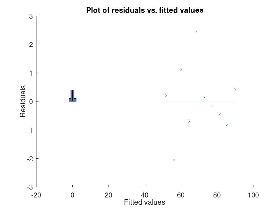
The lagged residual plot, useful for spotting autocorrelation. Twenty observations follow a slow oscillation layered on top of a linear trend, so consecutive residuals tend to be similar to one another. Plotting each residual against the one before it makes that pattern visible as a diagonal trend rather than a random scatter.
x = (1:20)'; y = 5 + 2*x + 4*sin (x*0.3); mdl = fitlm (x, y);
Each residual plotted against the residual immediately before it.
plotResiduals (mdl, 'lagged');
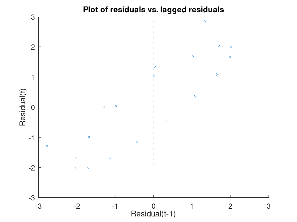
A normal probability plot of the residuals, using the carsmall data set. Fuel economy is modeled against vehicle weight. The probability plot sorts the residuals and compares them against a normal reference line, making departures from normality easy to spot at either tail.
load carsmall mdl = fitlm (Weight, MPG);
Normal probability plot of the residuals.
plotResiduals (mdl, 'probability');
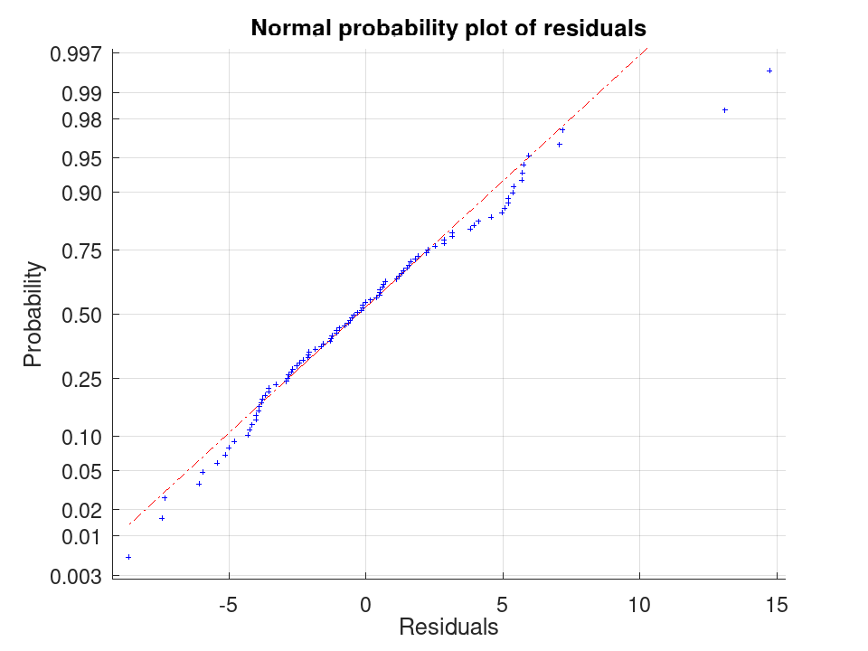
LinearModel: plotDiagnostics (mdl)
LinearModel: plotDiagnostics (mdl, plottype)
LinearModel: plotDiagnostics (mdl, plottype, Name, Value)
LinearModel: plotDiagnostics (ax, …)
LinearModel: h = plotDiagnostics (…)
plotDiagnostics (mdl) creates a case-order plot of the
leverage of each observation. The x-axis is the observation row number
running from 1 to the total number of rows including any excluded rows.
A dotted horizontal reference line marks the recommended threshold
2p/n, where p is mdl.NumCoefficients and n
is mdl.NumObservations.
plotDiagnostics (mdl, plottype) creates the diagnostic
plot specified by plottype. For all types except "contour",
the x-axis is the row number and covers all rows including excluded ones.
Excluded rows produce NaN values in the diagnostic vectors, which
appear as natural gaps in the plot with no special handling required.
plottype must be one of:
-
'leverage'(default) - Leverage of each observation (
mdl.Diagnostics.Leverage). One dotted horizontal reference line at 2p/n. Returns two handles:h(1)is the data scatter andh(2)is the reference line. -
'cookd' - Cook’s distance for each observation
(
mdl.Diagnostics.CooksDistance). One dotted reference line at 3 \times \mathrm{mean(CooksDistance)}, where the mean ignoresNaNvalues. Returns two handles:h(1)data,h(2)reference. -
'covratio' - Delete-1 ratio of the determinant of the coefficient covariance matrix
(
mdl.Diagnostics.CovRatio). Two dotted reference lines at 1 - 3p/n (lower bound) and 1 + 3p/n (upper bound). Both bounds are stored as a singleNaN-separated line object. Returns two handles:h(1)data,h(2)combined reference. -
'dfbetas' - Delete-1 scaled change in each coefficient estimate
(
mdl.Diagnostics.Dfbetas, one column per coefficient). One line object is drawn per coefficient. Two dotted reference lines at \pm 3/\sqrt{n} are stored as a singleNaN-separated line object. Returns p+1 handles:h(1)throughh(p)are the per-coefficient data lines andh(p+1)is the combined reference. Name-Value arguments are applied to all p data handles. -
'dffits' - Delete-1 scaled change in the fitted value
(
mdl.Diagnostics.Dffits). Two dotted reference lines at \pm 2\sqrt{p/n} stored as a singleNaN-separated line. Returns two handles:h(1)data,h(2)combined reference. -
's2_i' - Delete-1 variance estimate (
mdl.Diagnostics.S2_i). One dotted reference line atmdl.MSE. Returns two handles:h(1)data,h(2)reference. -
'contour' - Standardized residuals on the y-axis against leverage on the x-axis,
with Cook’s distance contours overlaid at levels
[0.05, 0.10, 0.15, 0.20, 0.25]. The contour surface is
computed on a 31-by-30 grid over the range of the active leverage and
residual values. Returns two handles:
h(1)is the data scatter (alineobject) andh(2)is the contour object.
plotDiagnostics (ax, …) targets the axes object
ax instead of the current axes returned by gca.
h = plotDiagnostics (…) returns a vector of graphics
handles. The number of handles depends on plottype as described
above. Name-Value arguments are applied to the data handle h(1),
except for "dfbetas" where they are applied to all p
coefficient handles. Reference line handles are never affected by
Name-Value arguments.
| Name | Description and default |
|---|---|
'Color' | Marker color for data points. For "dfbetas" this color is
applied to all p coefficient line objects.
Default: [0.1490 0.5490 0.8660]. |
'Marker' | Marker symbol. Any symbol accepted by plot is valid.
Default: 'x'. |
'MarkerSize' | Marker size in points. Default: 6. |
'MarkerEdgeColor' | Marker edge color. Default: 'auto'. |
'MarkerFaceColor' | Marker fill color. Default: 'none'. |
'LineWidth' | Width of the marker edge in points. Default: 0.5. |
The default leverage plot, and Cook's distance -- both flagging the same unusual observation. Ten students' exam scores are modeled against study hours, with one student whose hours and score are both far outside the rest of the group. With no arguments, plotDiagnostics plots each observation's leverage against its row number, with a dotted reference line at the conventional threshold 2*p/n. Passing 'cookd' instead shows each observation's overall influence on the fitted model.
Hours = [1;2;3;4;5;6;7;8;9;15]; Score = [52;55;61;64;70;73;77;81;85;130]; mdl = fitlm (Hours, Score);
Default: leverage of each observation.
plotDiagnostics (mdl);
Cook's distance, measuring each observation's overall influence.
plotDiagnostics (mdl, 'cookd');
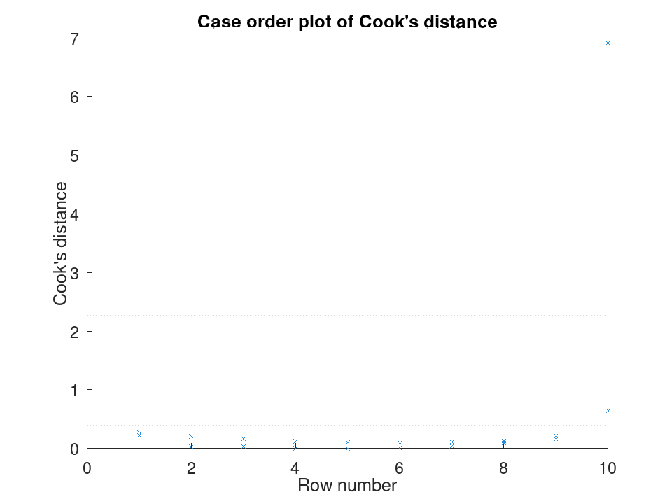
Delete-1 scaled change in each coefficient, one line per predictor. Ten observations depend on study hours and hours of sleep, with one observation whose sleep value and score are both unusually large. 'dfbetas' shows how much each coefficient estimate would change if that single observation were removed, scaled to be comparable across coefficients -- useful for seeing which specific predictor a given observation is most influential on.
Hours = [1;2;3;4;5;6;7;8;9;10]; Sleep = [5;6;5;7;6;8;7;9;8;20]; Score = [50;54;56;62;64;70;71;73;79;150]; mdl = fitlm ([Hours, Sleep], Score);
Scaled change in each coefficient if each observation were removed.
plotDiagnostics (mdl, 'dfbetas');
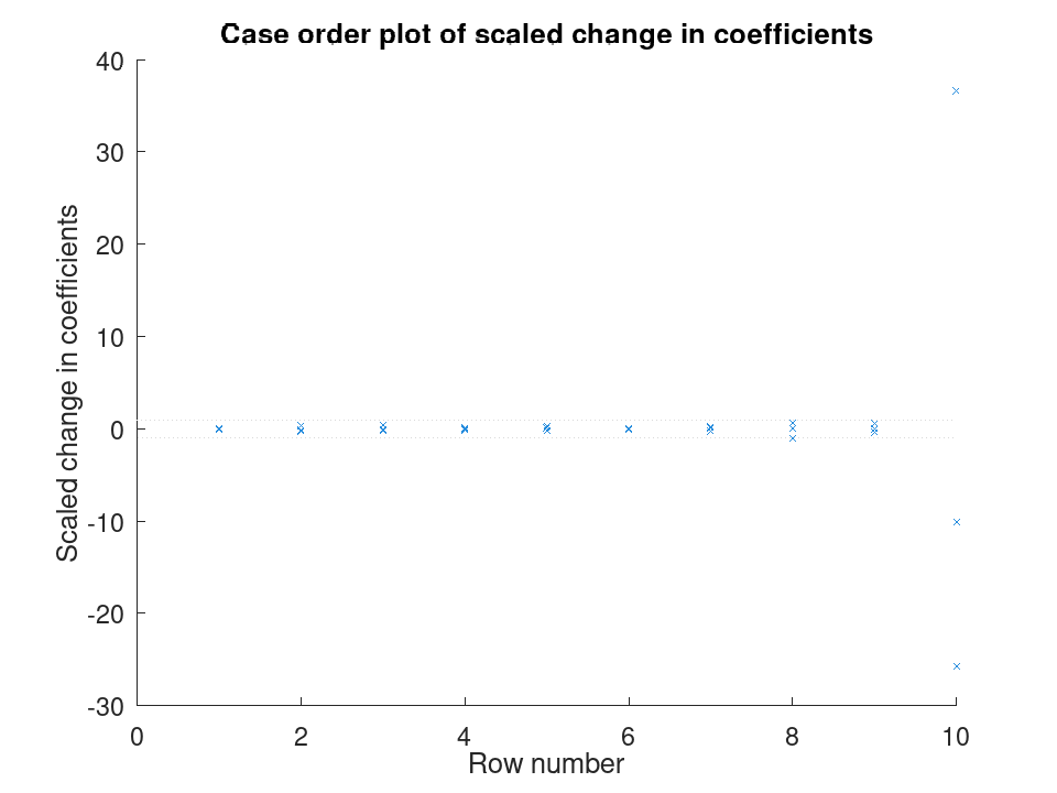
Delete-1 scaled change in the fitted value, using the carsmall data set. Fuel economy is modeled against vehicle weight. 'dffits' shows how much each observation's own fitted value would change if that observation were removed from the fit, with a dotted reference line at the conventional threshold 2*sqrt (p/n).
load carsmall mdl = fitlm (Weight, MPG);
Scaled change in the fitted value if each observation were removed.
plotDiagnostics (mdl, 'dffits');
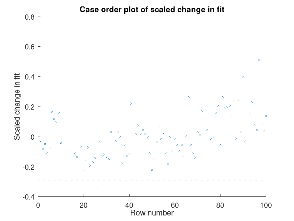
LinearModel: plotEffects (mdl)
LinearModel: plotEffects (ax, mdl)
LinearModel: h = plotEffects (…)
plotEffects (mdl) creates a horizontal dot-and-line plot
with one row per predictor. Each dot shows the estimated main effect on
the response from changing that predictor from its minimum observed value
to its maximum observed value, while holding all other predictors fixed
at their observed means. A horizontal line through each dot shows the
95% confidence interval for that effect.
The main effect for predictor xs is defined as g(x_{s,\max}) - g(x_{s,\min}), where the adjusted response function g evaluates the model at the specified value of xs with all other predictors set to their observed means. For numeric predictors the sign of the effect can be positive or negative depending on the direction of the relationship.
plotEffects (ax, mdl) creates the plot in the axes
object ax instead of the current axes returned by gca.
h = plotEffects (…) returns a vector of
p+1 graphics handles where p is the number of predictors.
h(1) is the line object containing the effect estimate markers
(one circle per predictor, plotted as a single line object with
XData of length p and YData = 1:p).
h(j+1) is the confidence interval line for predictor j,
with XData = [ci_lo, ci_hi] and YData = [j, j].
The y-axis tick labels follow the format
'varname: min to max', showing the predictor name and the
minimum and maximum observed values used to compute the effect.
The main effect and 95% confidence interval for each predictor. Ten observations depend on study hours and hours of sleep. plotEffects shows, for each predictor, how much the fitted response changes when that predictor moves from its observed minimum to its observed maximum, with all other predictors held at their observed means. The dotted vertical line marks zero effect.
Hours = [1;2;3;4;5;6;7;8;9;10]; Sleep = [5;6;5;7;6;8;7;6;8;7]; Score = [50;54;56;62;64;70;71;73;79;78]; mdl = fitlm ([Hours, Sleep], Score);
Main effect of each predictor, from its minimum to its maximum.
plotEffects (mdl);
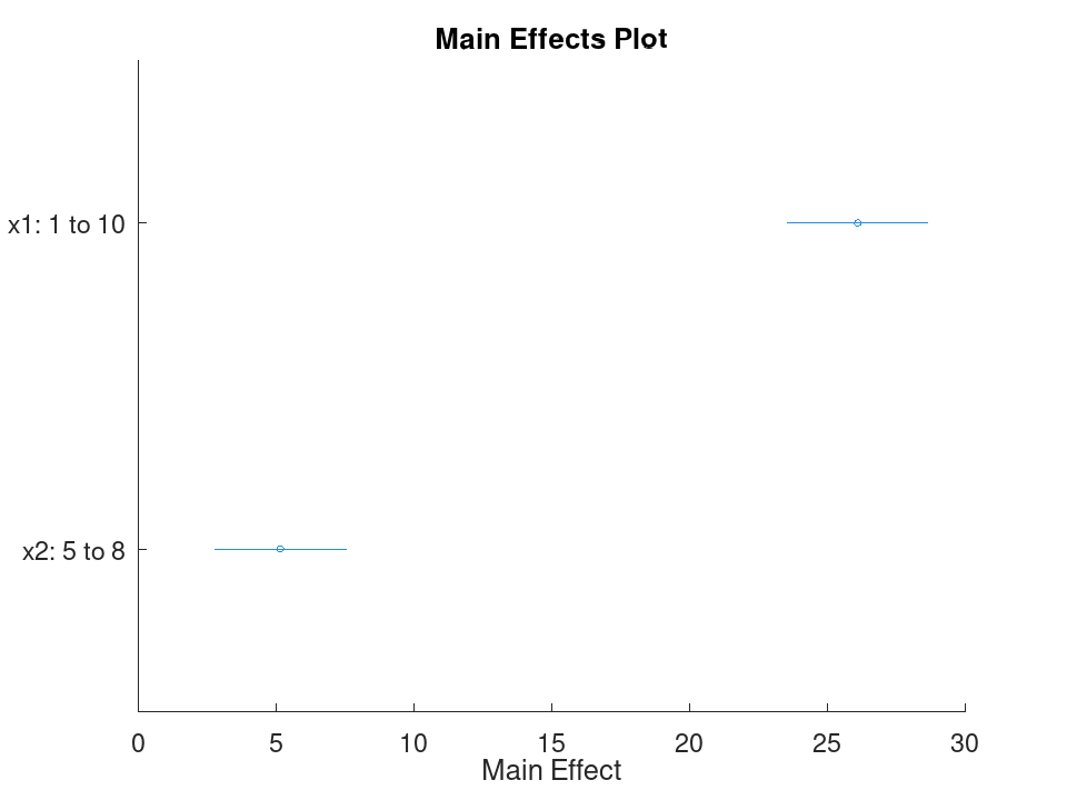
A categorical predictor's effect is shown the same way, labeled by its levels rather than a numeric range. Nine stores in three regions report ad spend and sales. The categorical Region gets a y-axis label showing its reference and comparison levels, just as a numeric predictor's label shows its minimum and maximum.
AdSpend = [10;20;30;15;25;35;12;22;32];
Region = {'North';'North';'North';'South';'South';'South'; ...
'East';'East';'East'};
Sales = [15;18;24;20;27;33;12;19;26];
T = table (AdSpend, Region, Sales);
mdl = fitlm (T, 'Sales ~ AdSpend + Region', 'CategoricalVars', {'Region'});
Main effect of AdSpend and of moving between Region levels.
plotEffects (mdl);
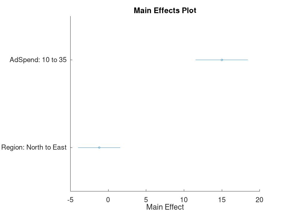
Comparing the main effects of four predictors at once, using the hald cement data set. Four chemical percentages in cement (ingredients) are used to predict heat given off while hardening (heat). With four correlated predictors and only 13 observations, several confidence intervals are wide enough to cross zero.
load hald mdl = fitlm (ingredients, heat);
Main effect of each of the four ingredients.
plotEffects (mdl);
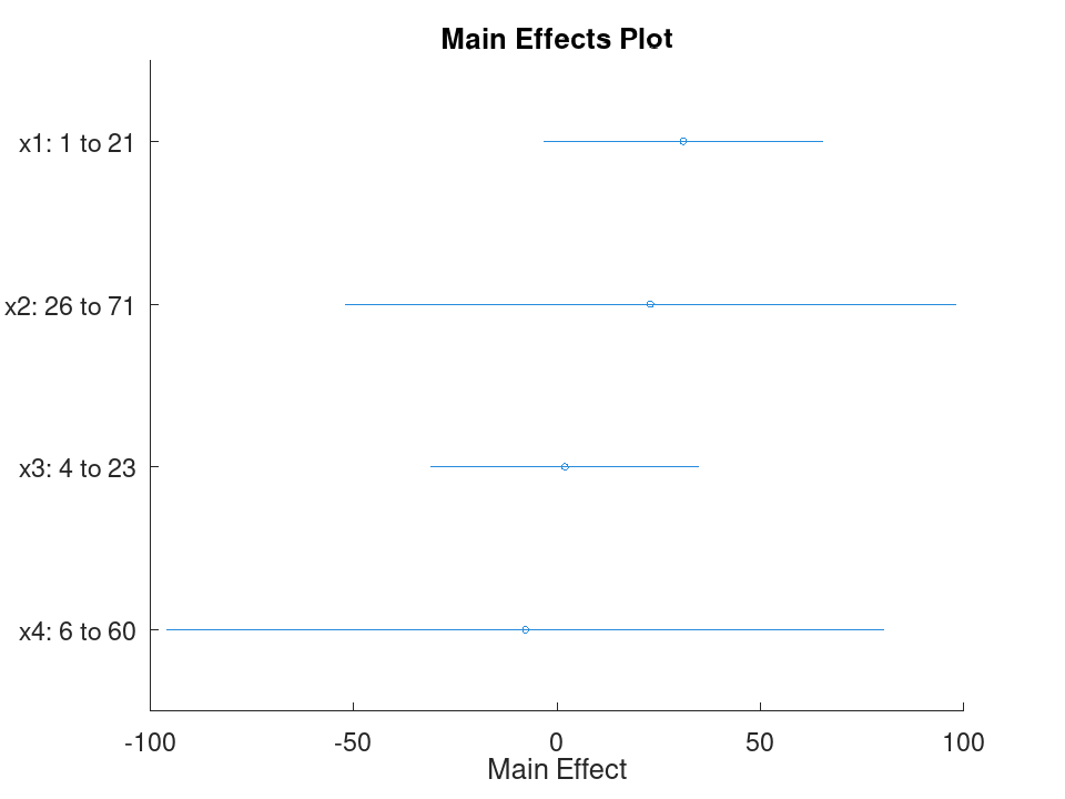
plotEffects on a CompactLinearModel gives the same plot as the original model. compact discards the training data but keeps everything plotEffects needs: the coefficient estimates, their covariance, and the effect contrasts computed at fit time.
Hours = [1;2;3;4;5;6;7;8;9;10]; Sleep = [5;6;5;7;6;8;7;6;8;7]; Score = [50;54;56;62;64;70;71;73;79;78]; mdl = fitlm ([Hours, Sleep], Score); cmdl = compact (mdl);
The same plot, produced from the compact model.
plotEffects (cmdl);
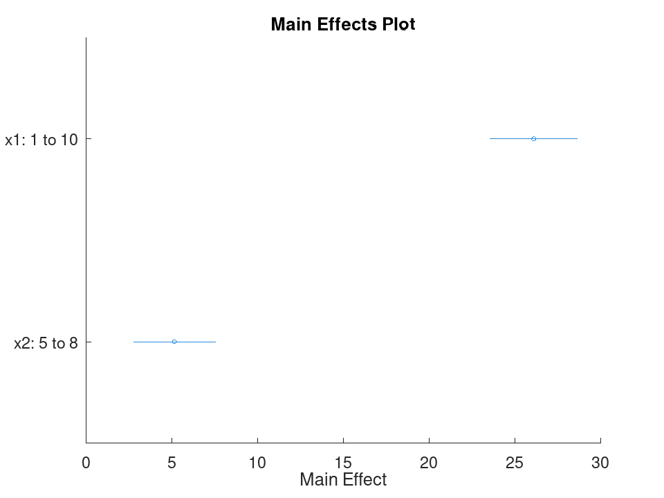
LinearModel: plotAdjustedResponse (mdl, var)
LinearModel: plotAdjustedResponse (mdl, var, Name, Value)
LinearModel: plotAdjustedResponse (ax, …)
LinearModel: h = plotAdjustedResponse (…)
plotAdjustedResponse (mdl, var) creates an adjusted
response plot for the predictor var in the linear regression
model mdl. var is a character vector or string naming a
predictor in mdl.PredictorNames, or a positive integer indexing
into mdl.VariableNames.
An adjusted response function describes the fitted response as a function of a single predictor, with the other predictors averaged out by averaging the fitted values over the observations used in the fit. For a model y_i = f (x_{1i}, x_{2i}, …, x_{pi}) + r_i, the adjusted response function for x_1 is g (x_1) = (1/n) \sum_{i=1}^n f (x_1, x_{2i}, x_{3i}, …, x_{pi}), where n is the number of observations used to fit the model. The adjusted response data value for observation i is \tilde y_i = g (x_{1i}) + r_i.
For a numeric predictor, the adjusted response function is evaluated on an evenly spaced grid of 100 points spanning the minimum to the maximum observed value of var. For a categorical predictor, the adjusted response function is evaluated at each category level.
Excluded or missing observations appear as NaN in the adjusted
data and produce gaps in the plotted data points.
plotAdjustedResponse (mdl, var, Name,
Value) specifies additional Name-Value arguments applied to the
adjusted data points (h(1)). The following are accepted:
| Name | Description and default |
|---|---|
'Color' | Marker color. Default: [0.1490 0.5490 0.8660]. |
'Marker' | Marker symbol. Default: 'x'. |
'MarkerSize' | Marker size in points. Default: 6. |
'MarkerEdgeColor' | Marker edge color. Default: 'auto'. |
'MarkerFaceColor' | Marker fill color. Default: 'none'. |
'LineWidth' | Width of the marker edge in points. Default: 0.5. |
plotAdjustedResponse (ax, …) plots into the axes
object ax instead of the current axes returned by gca.
h = plotAdjustedResponse (…) returns a 2-by-1
vector of line handles. h(1) corresponds to the adjusted
response data points and h(2) corresponds to the adjusted
response function. Name-Value arguments only affect h(1).
The adjusted response for one predictor, with the other predictor averaged out. Ten observations depend on study hours and hours of sleep. plotAdjustedResponse shows the fitted response as a function of x1 alone, with x2 held at its average observed value across the fit, alongside the actual adjusted data points (fitted value plus residual) for comparison.
Hours = [1;2;3;4;5;6;7;8;9;10]; Sleep = [5;6;5;7;6;8;7;6;8;7]; Score = [50;54;56;62;64;70;71;73;79;78]; mdl = fitlm ([Hours, Sleep], Score);
Adjusted response for x1, with x2 averaged out.
plotAdjustedResponse (mdl, 'x1');
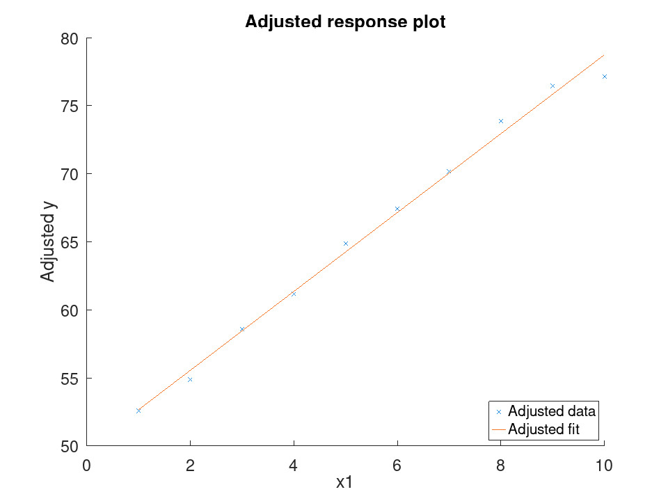
For a categorical predictor, the adjusted response function is evaluated at each level instead of a continuous grid. Nine stores in three regions report ad spend and sales. The adjusted response for Region is a step function through its three levels, with AdSpend averaged out.
AdSpend = [200;350;500;220;370;520;240;390;540];
Region = {'North';'North';'North';'South';'South';'South'; ...
'East';'East';'East'};
RegionEffect = [0;0;0;300;300;300;700;700;700];
Sales = 1000 + 0.5*AdSpend + RegionEffect + 5*sin ((1:9)');
T = table (AdSpend, Region, Sales);
mdl = fitlm (T, 'Sales ~ AdSpend + Region', 'CategoricalVars', {'Region'});
Adjusted response for Region, with AdSpend averaged out.
plotAdjustedResponse (mdl, 'Region');
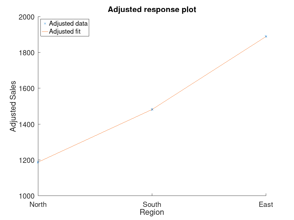
Isolating one predictor's adjusted response among several, using the hald cement data set. Four chemical percentages in cement (ingredients) are used to predict heat given off while hardening (heat). The adjusted response for the first ingredient is shown with the other three averaged out.
load hald mdl = fitlm (ingredients, heat);
Adjusted response for the first ingredient.
plotAdjustedResponse (mdl, 'x1');
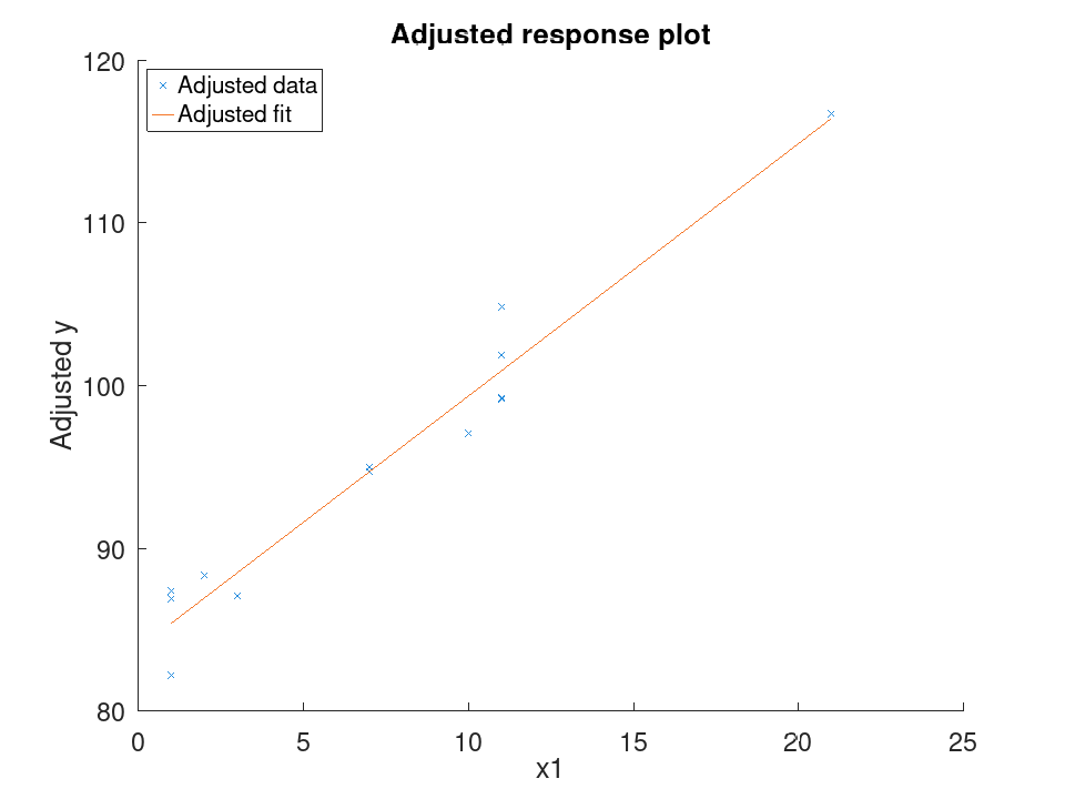
LinearModel: plotAdded (mdl)
LinearModel: plotAdded (mdl, coef)
LinearModel: plotAdded (mdl, coef, Name, Value)
LinearModel: plotAdded (ax, …)
LinearModel: h = plotAdded (…)
plotAdded (mdl) creates an added variable plot for the
whole model mdl except the constant (intercept) term.
plotAdded (mdl, coef) creates an added variable
plot for the coefficients specified by coef. coef is a
character vector or string naming a single coefficient in
mdl.CoefficientNames, the name of a categorical predictor in
mdl.PredictorNames (which selects that predictor’s whole group
of indicator coefficients), or a vector of positive integers indexing
into mdl.CoefficientNames.
An added variable plot, also known as a partial regression leverage plot, illustrates the incremental effect on the response of the selected terms after removing the effects of all other terms. For a single selected predictor x_1, the response y and x_1 are each fit to all other terms: y_i = g_y (x_{2i}, …, x_{pi}) + r_{yi}, x_{1i} = g_x (x_{2i}, …, x_{pi}) + r_{xi}. The adjusted values are \tilde y_i = \bar y + r_{yi} and \tilde x_{1i} = \bar x_1 + r_{xi}. When coef selects more than one coefficient, the selected columns of the design matrix are combined into a single direction using the unit vector u = \beta / \lVert \beta \rVert, and the added variable plot is created for that combined direction.
Excluded or missing observations appear as NaN in the adjusted
data and produce gaps in the plotted data points.
plotAdded (mdl, coef, Name, Value)
specifies additional Name-Value arguments applied to the adjusted data
points (h(1)). The following are accepted:
| Name | Description and default |
|---|---|
'Color' | Marker color. Default: [0.1490 0.5490 0.8660]. |
'Marker' | Marker symbol. Default: 'x'. |
'MarkerSize' | Marker size in points. Default: 6. |
'MarkerEdgeColor' | Marker edge color. Default: 'auto'. |
'MarkerFaceColor' | Marker fill color. Default: 'none'. |
'LineWidth' | Width of the marker edge in points. Default: 0.5. |
plotAdded (ax, …) plots into the axes object
ax instead of the current axes returned by gca.
h = plotAdded (…) returns a 3-by-1 vector of line
handles. h(1), h(2), and h(3) correspond to the
adjusted data points, the fitted line, and the 95% confidence bounds
of the fitted line, respectively. Name-Value arguments only affect
h(1).
Simple linear regression with a single predictor. Ten runners record their weekly training distance and their finish time in a 10k race. We fit a straight line through this data and look at the fitted coefficients, then use predict to estimate the finish time for a runner who trains a distance not in the sample.
Distance = [10; 15; 20; 25; 30; 35; 40; 45; 50; 55]; Time = [58; 55; 52; 50; 47; 45; 43; 41; 40; 38]; X = Distance; y = Time;
Fit the model and inspect the estimated slope and intercept.
mdl = fitlm (X, y)
mdl =
Linear regression model:
y ~ 1 + x1
Estimated Coefficients:
2x4 table
Estimate SE tStat pValue
________ _________ ________ ___________
(Intercept) 61.2 0.654588 93.494 1.91213e-13
x1 -0.44 0.0184226 -23.8836 1.00609e-08
Number of observations: 10, Error degrees of freedom: 8
Root Mean Squared Error: 0.83666
R-squared: 0.986169, Adjusted R-Squared: 0.984441
F-statistic vs. constant model: 570.429, p-value = 1.00609e-08
Predict the finish time for a runner training 32 km per week.
ypred = predict (mdl, 32)
ypred = 47.120
Multiple linear regression with two predictors, followed by a confidence interval on the coefficients. Thirteen coffee shops report their weekly foot traffic and the number of items on their menu, along with weekly revenue. We fit a model with both predictors, then use coefCI to see how precisely each coefficient is estimated.
Traffic = [120; 150; 90; 200; 175; 60; 220; 140; 100; 190; 80; 210; 130];
MenuSize = [8; 12; 6; 15; 10; 5; 18; 9; 7; 14; 6; 16; 11];
Revenue = [1450; 1820; 1010; 2400; 2050; 700; 2650; 1700; 1150; ...
2300; 900; 2500; 1600];
X = [Traffic, MenuSize];
y = Revenue;
Fit the model with both predictors together.
mdl = fitlm (X, y)
mdl =
Linear regression model:
y ~ 1 + x1 + x2
Estimated Coefficients:
3x4 table
Estimate SE tStat pValue
________ ________ ________ ___________
(Intercept) -47.0932 27.3456 -1.72215 0.115771
x1 11.4079 0.616078 18.517 4.55169e-09
x2 11.4344 7.68384 1.48811 0.167562
Number of observations: 13, Error degrees of freedom: 10
Root Mean Squared Error: 32.4551
R-squared: 0.997901, Adjusted R-Squared: 0.997482
F-statistic vs. constant model: 2377.53, p-value = 4.07061e-14
Check how tight the 95% confidence interval is on each coefficient.
ci = coefCI (mdl)
ci =
-108.0231 13.8366
10.0352 12.7806
-5.6862 28.5551
Growing a model with addTerms and predicting with the richer model. We model fuel economy from the carsmall data set using weight and horsepower as main effects only. addTerms then brings in the weight-horsepower interaction without needing to refit by hand, and predict shows how the estimate for a new car changes once that interaction is included.
load carsmall X = [Weight, Horsepower]; y = MPG;
Fit the additive model first.
mdl = fitlm (X, y);
Add the interaction between weight and horsepower.
mdl2 = addTerms (mdl, 'x1:x2');
Compare predictions from both models for the same new car.
Xnew = [3200, 120]; ypred1 = predict (mdl, Xnew)
ypred1 = 21.719
ypred2 = predict (mdl2, Xnew)
ypred2 = 20.416
Simplifying a model with removeTerms and comparing fit quality. We fit the full Hald cement model with all four ingredients, then use removeTerms to drop the weakest predictor and refit automatically. Comparing SSE before and after shows how little explanatory power that ingredient was actually contributing.
load hald X = ingredients; y = heat;
Fit the model with all four ingredients.
mdl = fitlm (X, y);
Drop the third ingredient and refit on the same data.
mdl2 = removeTerms (mdl, 'x3');
Compare how much the error sum of squares changed.
sse_full = mdl.SSE
sse_full = 47.864
sse_reduced = mdl2.SSE
sse_reduced = 47.973
Testing a linear hypothesis and checking residual autocorrelation. Twelve patients are given a drug at different doses over different treatment durations, and a recovery score is recorded. coefTest checks whether the dose and duration coefficients are actually equal, and dwtest separately checks whether the residuals still carry a leftover pattern the model failed to capture.
Dose = [10; 15; 20; 25; 30; 35; 12; 18; 22; 28; 32; 38]; Duration = [5; 7; 9; 11; 13; 15; 6; 8; 10; 12; 14; 16]; Recovery = [42; 48; 55; 60; 68; 74; 45; 52; 58; 65; 71; 78]; X = [Dose, Duration]; y = Recovery; mdl = fitlm (X, y);
Test H0: the Dose and Duration coefficients are equal.
H = [0 1 -1]; [p, F, r] = coefTest (mdl, H)
p = 0.3535 F = 0.9571 r = 1
Check for autocorrelation left over in the residuals.
[pdw, dw] = dwtest (mdl)
pdw = 0.3658 dw = 2.4432
Checking residuals against fitted values. We fit a mileage model on the carsmall data set using weight and horsepower, then plot the raw residuals against the fitted values. A pattern in this plot, rather than a random scatter, would suggest the linear model is missing some curvature in the relationship.
load carsmall X = [Weight, Horsepower]; y = MPG; mdl = fitlm (X, y); plotResiduals (mdl, 'fitted')
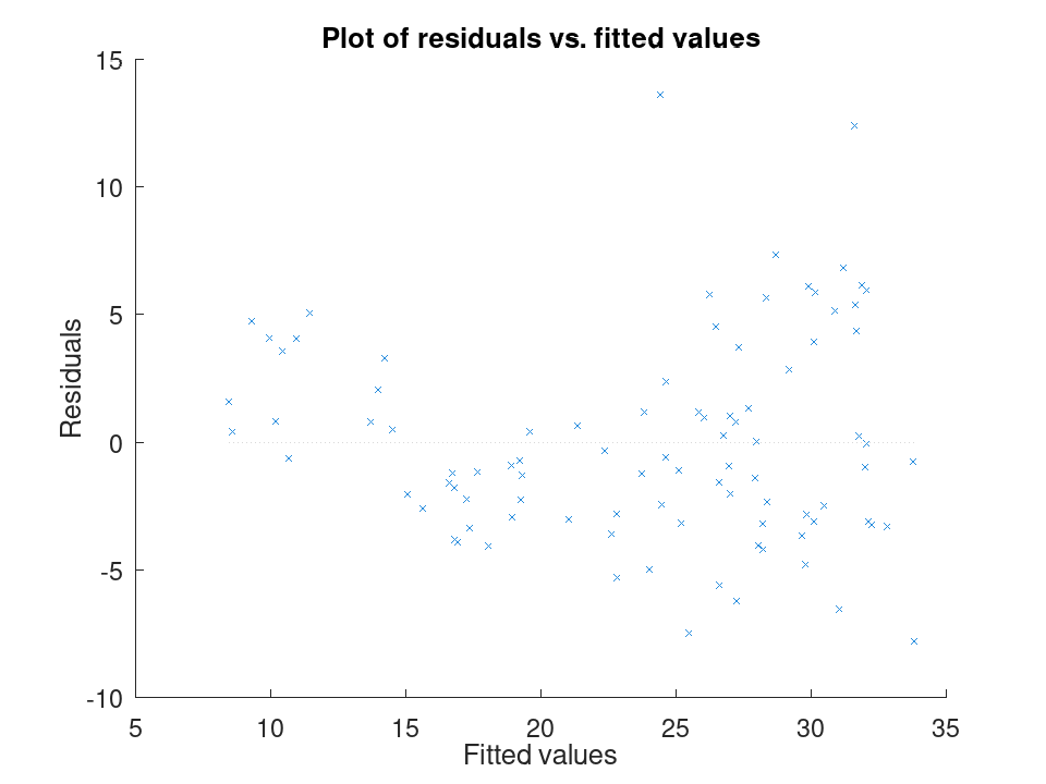
Spotting influential observations with Cook's distance. Sixteen houses are matched by size and age to a sale price, but one house was sold far above what its size and age would predict. After fitting the model, plotDiagnostics with the cookd option highlights that single observation as having outsized influence on the fit.
Size = [80; 95; 110; 120; 65; 140; 100; 130; 90; 150; 75; 105; ...
115; 85; 135; 125];
Age = [5; 10; 3; 8; 20; 2; 15; 6; 12; 1; 18; 9; 4; 14; 7; 11];
Price = [200; 230; 260; 280; 150; 320; 240; 300; 210; 340; 170; ...
250; 270; 190; 500; 290];
X = [Size, Age];
y = Price;
mdl = fitlm (X, y);
plotDiagnostics (mdl, 'cookd')
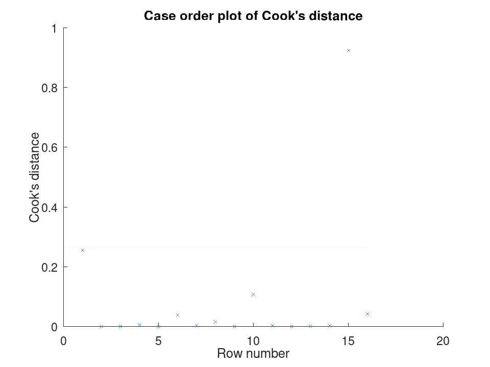
Comparing the size of each predictor's effect, alongside a hypothesis test on the model as a whole. We fit a mileage model on the carsmall data set using weight and horsepower. plotEffects draws each coefficient's estimate with its confidence interval side by side, and coefTest checks whether weight's effect is significantly different from horsepower's.
load carsmall X = [Weight, Horsepower]; y = MPG; mdl = fitlm (X, y);
Visualize the relative size of each predictor's effect.
plotEffects (mdl)
Test whether the two coefficients differ significantly.
H = [0 1 -1]; [p, F, r] = coefTest (mdl, H)
p = 0.073643 F = 3.2759 r = 1
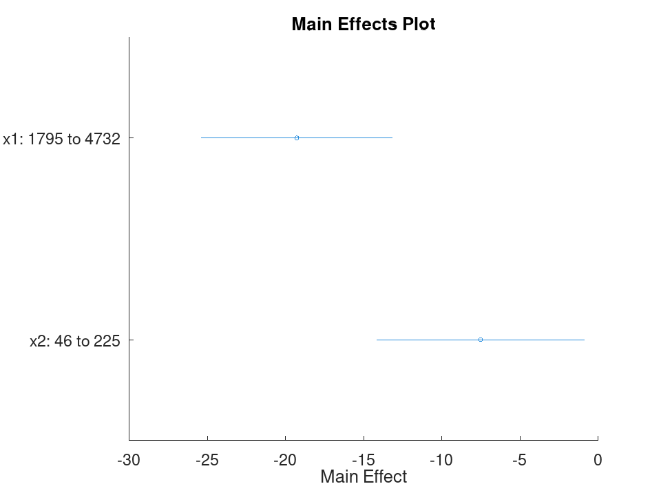
LinearModel: plot (mdl)
LinearModel: plot (ax, mdl)
LinearModel: h = plot (…)
plot (mdl) creates a plot whose type depends on the
number of predictors in mdl. If mdl has two or more
predictors, plot creates an added variable plot for the whole
model except the constant (intercept) term, equivalent to
plotAdded (mdl). If mdl has exactly one
predictor, plot creates a scatter plot of the data together
with the fitted curve and its 95% confidence bounds. If mdl
has no predictors, plot creates a histogram of the residuals,
equivalent to plotResiduals (mdl).
For the single-predictor case, the fitted curve and confidence
bounds are computed with predict, evaluated at 100 equally
spaced points spanning the observed range of the predictor when the
predictor is numeric, or at each level of the predictor when it is
categorical. Excluded or missing observations appear as NaN
in the data and produce gaps in the plotted points.
plot (ax, mdl) plots into the axes object
ax instead of the current axes returned by gca.
h = plot (…) returns a vector of graphics object
handles. For the two-or-more-predictor and no-predictor cases, see
plotAdded and plotResiduals, respectively, for the
meaning of h. For the single-predictor case, h(1),
h(2), and h(3) correspond to the data points, the fitted
curve, and the 95% confidence bounds of the fitted curve,
respectively.
Simple linear regression with a single predictor. Ten runners record their weekly training distance and their finish time in a 10k race. We fit a straight line through this data and look at the fitted coefficients, then use predict to estimate the finish time for a runner who trains a distance not in the sample.
Distance = [10; 15; 20; 25; 30; 35; 40; 45; 50; 55]; Time = [58; 55; 52; 50; 47; 45; 43; 41; 40; 38]; X = Distance; y = Time;
Fit the model and inspect the estimated slope and intercept.
mdl = fitlm (X, y)
mdl =
Linear regression model:
y ~ 1 + x1
Estimated Coefficients:
2x4 table
Estimate SE tStat pValue
________ _________ ________ ___________
(Intercept) 61.2 0.654588 93.494 1.91213e-13
x1 -0.44 0.0184226 -23.8836 1.00609e-08
Number of observations: 10, Error degrees of freedom: 8
Root Mean Squared Error: 0.83666
R-squared: 0.986169, Adjusted R-Squared: 0.984441
F-statistic vs. constant model: 570.429, p-value = 1.00609e-08
Predict the finish time for a runner training 32 km per week.
ypred = predict (mdl, 32)
ypred = 47.120
Multiple linear regression with two predictors, followed by a confidence interval on the coefficients. Thirteen coffee shops report their weekly foot traffic and the number of items on their menu, along with weekly revenue. We fit a model with both predictors, then use coefCI to see how precisely each coefficient is estimated.
Traffic = [120; 150; 90; 200; 175; 60; 220; 140; 100; 190; 80; 210; 130];
MenuSize = [8; 12; 6; 15; 10; 5; 18; 9; 7; 14; 6; 16; 11];
Revenue = [1450; 1820; 1010; 2400; 2050; 700; 2650; 1700; 1150; ...
2300; 900; 2500; 1600];
X = [Traffic, MenuSize];
y = Revenue;
Fit the model with both predictors together.
mdl = fitlm (X, y)
mdl =
Linear regression model:
y ~ 1 + x1 + x2
Estimated Coefficients:
3x4 table
Estimate SE tStat pValue
________ ________ ________ ___________
(Intercept) -47.0932 27.3456 -1.72215 0.115771
x1 11.4079 0.616078 18.517 4.55169e-09
x2 11.4344 7.68384 1.48811 0.167562
Number of observations: 13, Error degrees of freedom: 10
Root Mean Squared Error: 32.4551
R-squared: 0.997901, Adjusted R-Squared: 0.997482
F-statistic vs. constant model: 2377.53, p-value = 4.07061e-14
Check how tight the 95% confidence interval is on each coefficient.
ci = coefCI (mdl)
ci =
-108.0231 13.8366
10.0352 12.7806
-5.6862 28.5551
Growing a model with addTerms and predicting with the richer model. We model fuel economy from the carsmall data set using weight and horsepower as main effects only. addTerms then brings in the weight-horsepower interaction without needing to refit by hand, and predict shows how the estimate for a new car changes once that interaction is included.
load carsmall X = [Weight, Horsepower]; y = MPG;
Fit the additive model first.
mdl = fitlm (X, y);
Add the interaction between weight and horsepower.
mdl2 = addTerms (mdl, 'x1:x2');
Compare predictions from both models for the same new car.
Xnew = [3200, 120]; ypred1 = predict (mdl, Xnew)
ypred1 = 21.719
ypred2 = predict (mdl2, Xnew)
ypred2 = 20.416
Simplifying a model with removeTerms and comparing fit quality. We fit the full Hald cement model with all four ingredients, then use removeTerms to drop the weakest predictor and refit automatically. Comparing SSE before and after shows how little explanatory power that ingredient was actually contributing.
load hald X = ingredients; y = heat;
Fit the model with all four ingredients.
mdl = fitlm (X, y);
Drop the third ingredient and refit on the same data.
mdl2 = removeTerms (mdl, 'x3');
Compare how much the error sum of squares changed.
sse_full = mdl.SSE
sse_full = 47.864
sse_reduced = mdl2.SSE
sse_reduced = 47.973
Testing a linear hypothesis and checking residual autocorrelation. Twelve patients are given a drug at different doses over different treatment durations, and a recovery score is recorded. coefTest checks whether the dose and duration coefficients are actually equal, and dwtest separately checks whether the residuals still carry a leftover pattern the model failed to capture.
Dose = [10; 15; 20; 25; 30; 35; 12; 18; 22; 28; 32; 38]; Duration = [5; 7; 9; 11; 13; 15; 6; 8; 10; 12; 14; 16]; Recovery = [42; 48; 55; 60; 68; 74; 45; 52; 58; 65; 71; 78]; X = [Dose, Duration]; y = Recovery; mdl = fitlm (X, y);
Test H0: the Dose and Duration coefficients are equal.
H = [0 1 -1]; [p, F, r] = coefTest (mdl, H)
p = 0.3535 F = 0.9571 r = 1
Check for autocorrelation left over in the residuals.
[pdw, dw] = dwtest (mdl)
pdw = 0.3658 dw = 2.4432
Checking residuals against fitted values. We fit a mileage model on the carsmall data set using weight and horsepower, then plot the raw residuals against the fitted values. A pattern in this plot, rather than a random scatter, would suggest the linear model is missing some curvature in the relationship.
load carsmall X = [Weight, Horsepower]; y = MPG; mdl = fitlm (X, y); plotResiduals (mdl, 'fitted')
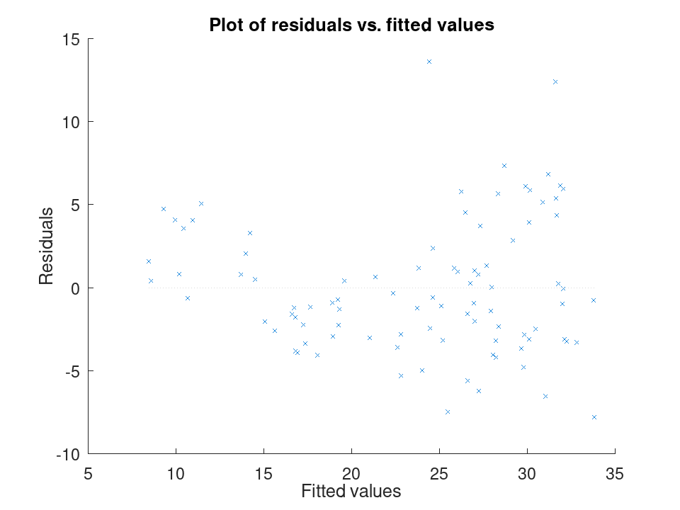
Spotting influential observations with Cook's distance. Sixteen houses are matched by size and age to a sale price, but one house was sold far above what its size and age would predict. After fitting the model, plotDiagnostics with the cookd option highlights that single observation as having outsized influence on the fit.
Size = [80; 95; 110; 120; 65; 140; 100; 130; 90; 150; 75; 105; ...
115; 85; 135; 125];
Age = [5; 10; 3; 8; 20; 2; 15; 6; 12; 1; 18; 9; 4; 14; 7; 11];
Price = [200; 230; 260; 280; 150; 320; 240; 300; 210; 340; 170; ...
250; 270; 190; 500; 290];
X = [Size, Age];
y = Price;
mdl = fitlm (X, y);
plotDiagnostics (mdl, 'cookd')
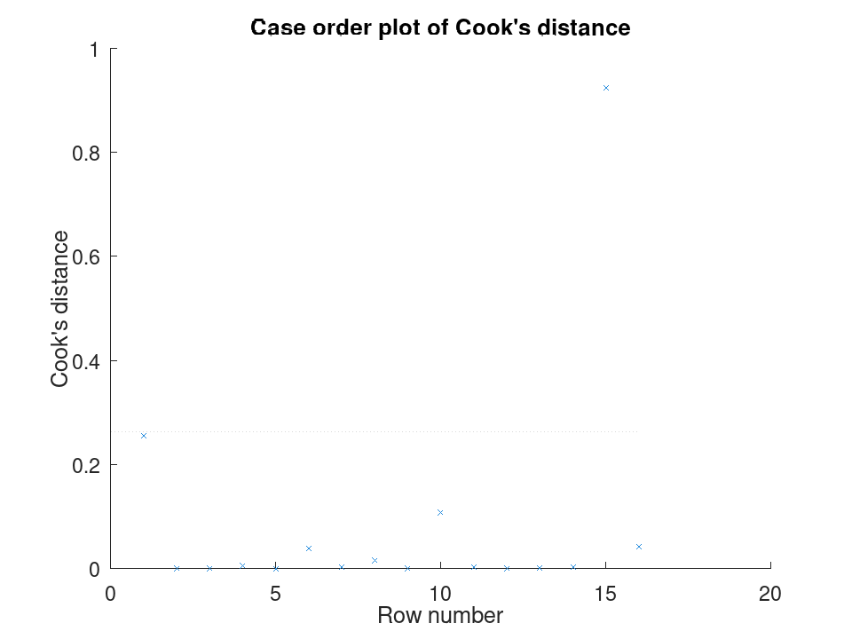
Comparing the size of each predictor's effect, alongside a hypothesis test on the model as a whole. We fit a mileage model on the carsmall data set using weight and horsepower. plotEffects draws each coefficient's estimate with its confidence interval side by side, and coefTest checks whether weight's effect is significantly different from horsepower's.
load carsmall X = [Weight, Horsepower]; y = MPG; mdl = fitlm (X, y);
Visualize the relative size of each predictor's effect.
plotEffects (mdl)
Test whether the two coefficients differ significantly.
H = [0 1 -1]; [p, F, r] = coefTest (mdl, H)
p = 0.073643 F = 3.2759 r = 1
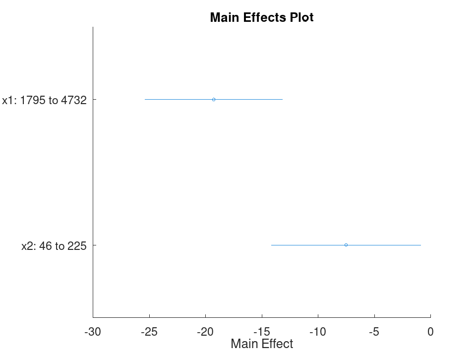
LinearModel: plotInteraction (mdl, var1, var2)
LinearModel: plotInteraction (mdl, var1, var2, ptype)
LinearModel: plotInteraction (ax, …)
LinearModel: h = plotInteraction (…)
plotInteraction (mdl, var1, var2) creates a
plot of the main effects of var1 and var2 together with
their conditional effects, with horizontal lines through each effect
value indicating its 95% confidence interval. var1 and
var2 are each a character vector or string naming a variable in
mdl.VariableNames, or a positive integer indexing into
mdl.VariableNames; neither may name the response variable, and
they must be different variables.
The main effect of a predictor is the change in the adjusted response between the two predictor values that produce the minimum and maximum adjusted response, with the other predictor averaged over its own observed values row by row. For a numeric predictor these two values are its observed minimum and maximum; for a categorical predictor every level is evaluated and the levels producing the minimum and maximum adjusted response are used, so the effect is always nonnegative.
The conditional effect of var1 is its effect recomputed with var2 additionally held fixed at each of a small set of conditioning values, and likewise the conditional effect of var2 holds var1 fixed. The conditioning values are the observed minimum, mean of the minimum and maximum, and maximum for a numeric predictor, or every level for a categorical predictor. When the main effect and conditional effect points for a predictor do not align vertically, the model exhibits an interaction between var1 and var2.
plotInteraction (mdl, var1, var2, ptype)
selects the plot type. ptype is 'effects' (default), as
described above, or 'predictions', which instead plots the
adjusted response as a function of var2 for each conditioning
value of var1 held fixed, evaluated over 101 equally spaced
points spanning the observed range of var2 when var2 is
numeric, or at each level of var2 when it is categorical.
plotInteraction (ax, …) plots into the axes object
ax instead of the current axes returned by gca.
h = plotInteraction (…) returns a vector of line
handles. When ptype is 'effects', h(1) is the
marker line through the two main effect points, h(2) and
h(3) are the confidence interval lines for the main effects of
var1 and var2, and the remaining entries are the
conditional effect points and their confidence intervals, tagged
'conditional1' for var1 and 'conditional2' for
var2. The main effect line objects are tagged 'main'.
When ptype is 'predictions', each entry in h
corresponds to one adjusted response curve, one per conditioning
value of var1.
The main effect and conditional effects of two predictors, the default 'effects' plot. Ten observations depend on study hours and hours of sleep, fit with an interaction term. For each predictor, the top marker is its main effect; the markers below it are its effect recomputed with the other predictor held fixed at a few conditioning values. When those markers do not line up vertically, the predictors interact.
Hours = [1;2;3;4;5;6;7;8;9;10]; Sleep = [5;6;5;7;6;8;7;6;8;7]; Score = [50;54;56;62;64;70;71;73;79;78]; mdl = fitlm ([Hours, Sleep], Score, 'y ~ x1*x2');
Main and conditional effects of x1 and x2.
plotInteraction (mdl, 'x1', 'x2');
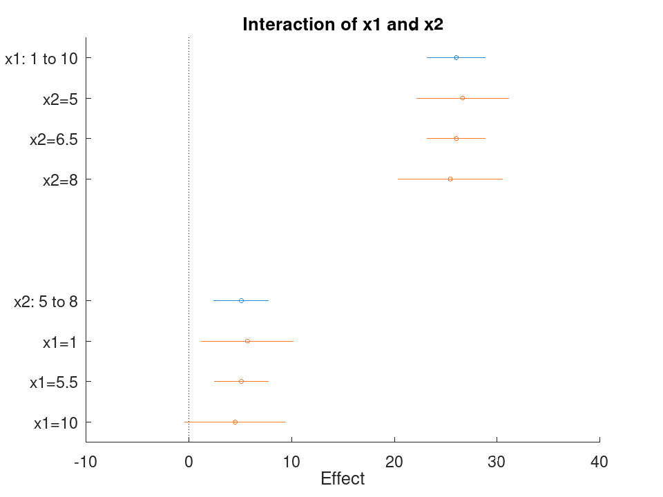
The 'predictions' plot type: adjusted response curves for x2, one per conditioning value of x1. Reusing the same interaction model, each curve shows how the adjusted response changes with x2, holding x1 fixed at a different value. Curves with different slopes indicate an interaction; parallel curves would indicate none.
Hours = [1;2;3;4;5;6;7;8;9;10]; Sleep = [5;6;5;7;6;8;7;6;8;7]; Score = [50;54;56;62;64;70;71;73;79;78]; mdl = fitlm ([Hours, Sleep], Score, 'y ~ x1*x2');
Adjusted response vs. x2, for three fixed values of x1.
plotInteraction (mdl, 'x1', 'x2', 'predictions');
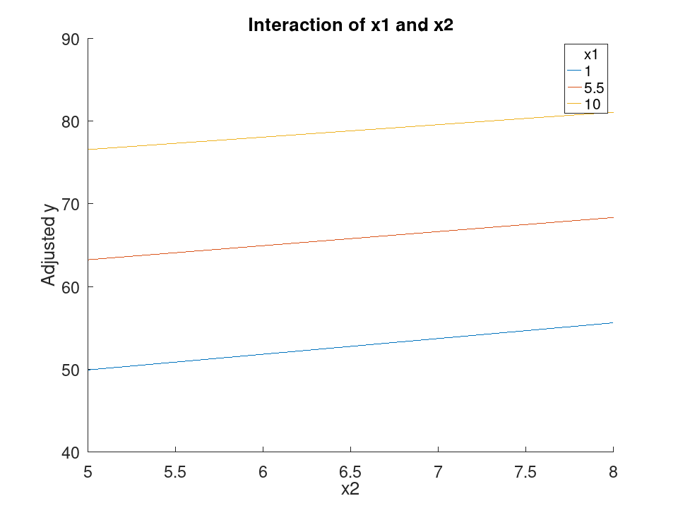
A categorical predictor's main and conditional effects, alongside a numeric one. Nine stores in three regions report ad spend and sales, fit with an interaction between AdSpend and Region. The categorical predictor's conditional effects are shown once per level rather than at a handful of numeric conditioning points.
AdSpend = [10;20;30;15;25;35;12;22;32];
Region = {'North';'North';'North';'South';'South';'South'; ...
'East';'East';'East'};
Sales = [15;18;24;20;27;33;12;19;26];
T = table (AdSpend, Region, Sales);
mdl = fitlm (T, 'Sales ~ AdSpend*Region', 'CategoricalVars', {'Region'});
Main and conditional effects of AdSpend and Region.
plotInteraction (mdl, 'AdSpend', 'Region');
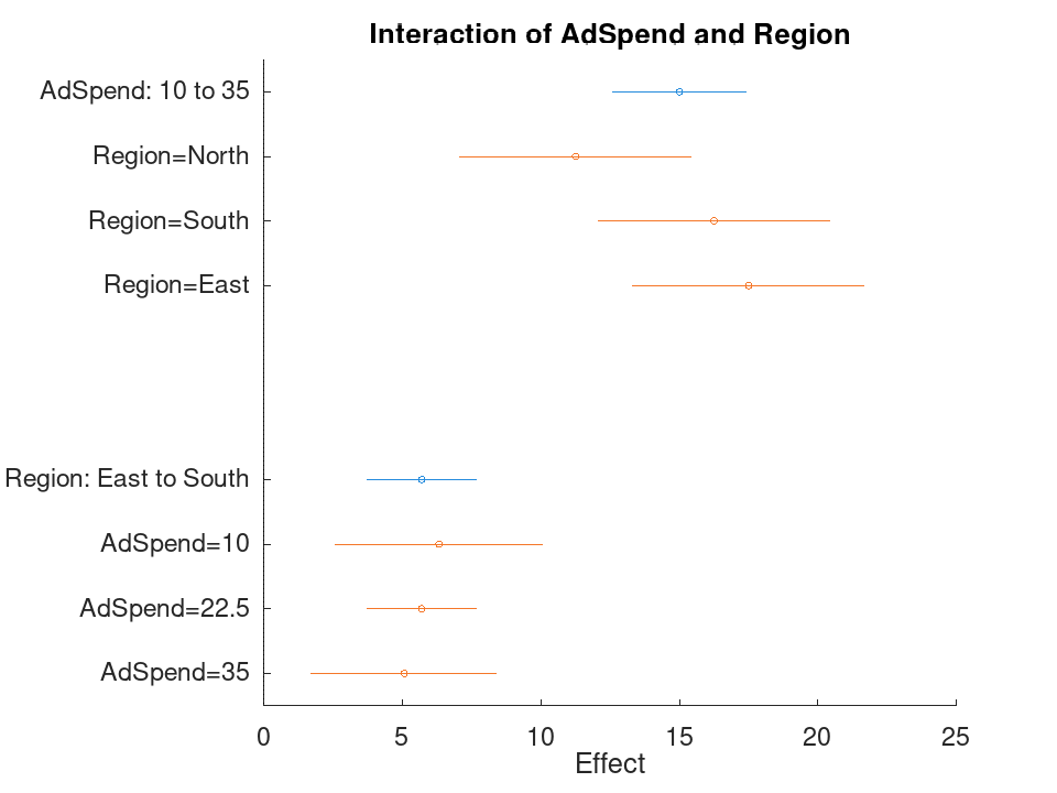
plotInteraction on a CompactLinearModel gives the same plot as the original model. compact discards the training data but keeps everything plotInteraction needs: the coefficient estimates, their covariance, and the interaction contrasts computed at fit time.
Hours = [1;2;3;4;5;6;7;8;9;10]; Sleep = [5;6;5;7;6;8;7;6;8;7]; Score = [50;54;56;62;64;70;71;73;79;78]; mdl = fitlm ([Hours, Sleep], Score, 'y ~ x1*x2'); cmdl = compact (mdl);
The same plot, produced from the compact model.
plotInteraction (cmdl, 'x1', 'x2');
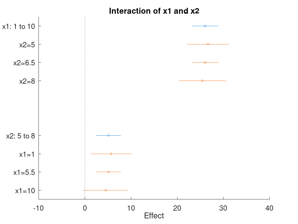
LinearModel: cmdl = compact (mdl)
cmdl = compact (mdl) returns a
CompactLinearModel object that retains the coefficient
estimates, coefficient covariance, fit statistics, model formula, and
fitting method information of mdl, but discards the training
data and everything derived from it. Specifically, the following
properties of mdl are not carried over and are unavailable on
cmdl: Fitted, Residuals, Diagnostics,
ObservationInfo, ObservationNames, Variables,
Steps, and ModelFitVsNullModel.
If mdl was fit using robust regression, the Robust
structure is retained on cmdl except for its Weights
field, which is always emptied; RobustWgtFun and Tune
are preserved unchanged.
A CompactLinearModel object consumes less memory than a
LinearModel object and can still be used with predict,
feval, random, coefCI, and coefTest, but
does not support methods that require the original training data or
refitting, such as addTerms, removeTerms, step,
and dwtest.
See also: LinearModel, CompactLinearModel
Simple linear regression with a single predictor. Ten runners record their weekly training distance and their finish time in a 10k race. We fit a straight line through this data and look at the fitted coefficients, then use predict to estimate the finish time for a runner who trains a distance not in the sample.
Distance = [10; 15; 20; 25; 30; 35; 40; 45; 50; 55]; Time = [58; 55; 52; 50; 47; 45; 43; 41; 40; 38]; X = Distance; y = Time;
Fit the model and inspect the estimated slope and intercept.
mdl = fitlm (X, y)
mdl =
Linear regression model:
y ~ 1 + x1
Estimated Coefficients:
2x4 table
Estimate SE tStat pValue
________ _________ ________ ___________
(Intercept) 61.2 0.654588 93.494 1.91213e-13
x1 -0.44 0.0184226 -23.8836 1.00609e-08
Number of observations: 10, Error degrees of freedom: 8
Root Mean Squared Error: 0.83666
R-squared: 0.986169, Adjusted R-Squared: 0.984441
F-statistic vs. constant model: 570.429, p-value = 1.00609e-08
Predict the finish time for a runner training 32 km per week.
ypred = predict (mdl, 32)
ypred = 47.120
Multiple linear regression with two predictors, followed by a confidence interval on the coefficients. Thirteen coffee shops report their weekly foot traffic and the number of items on their menu, along with weekly revenue. We fit a model with both predictors, then use coefCI to see how precisely each coefficient is estimated.
Traffic = [120; 150; 90; 200; 175; 60; 220; 140; 100; 190; 80; 210; 130];
MenuSize = [8; 12; 6; 15; 10; 5; 18; 9; 7; 14; 6; 16; 11];
Revenue = [1450; 1820; 1010; 2400; 2050; 700; 2650; 1700; 1150; ...
2300; 900; 2500; 1600];
X = [Traffic, MenuSize];
y = Revenue;
Fit the model with both predictors together.
mdl = fitlm (X, y)
mdl =
Linear regression model:
y ~ 1 + x1 + x2
Estimated Coefficients:
3x4 table
Estimate SE tStat pValue
________ ________ ________ ___________
(Intercept) -47.0932 27.3456 -1.72215 0.115771
x1 11.4079 0.616078 18.517 4.55169e-09
x2 11.4344 7.68384 1.48811 0.167562
Number of observations: 13, Error degrees of freedom: 10
Root Mean Squared Error: 32.4551
R-squared: 0.997901, Adjusted R-Squared: 0.997482
F-statistic vs. constant model: 2377.53, p-value = 4.07061e-14
Check how tight the 95% confidence interval is on each coefficient.
ci = coefCI (mdl)
ci =
-108.0231 13.8366
10.0352 12.7806
-5.6862 28.5551
Growing a model with addTerms and predicting with the richer model. We model fuel economy from the carsmall data set using weight and horsepower as main effects only. addTerms then brings in the weight-horsepower interaction without needing to refit by hand, and predict shows how the estimate for a new car changes once that interaction is included.
load carsmall X = [Weight, Horsepower]; y = MPG;
Fit the additive model first.
mdl = fitlm (X, y);
Add the interaction between weight and horsepower.
mdl2 = addTerms (mdl, 'x1:x2');
Compare predictions from both models for the same new car.
Xnew = [3200, 120]; ypred1 = predict (mdl, Xnew)
ypred1 = 21.719
ypred2 = predict (mdl2, Xnew)
ypred2 = 20.416
Simplifying a model with removeTerms and comparing fit quality. We fit the full Hald cement model with all four ingredients, then use removeTerms to drop the weakest predictor and refit automatically. Comparing SSE before and after shows how little explanatory power that ingredient was actually contributing.
load hald X = ingredients; y = heat;
Fit the model with all four ingredients.
mdl = fitlm (X, y);
Drop the third ingredient and refit on the same data.
mdl2 = removeTerms (mdl, 'x3');
Compare how much the error sum of squares changed.
sse_full = mdl.SSE
sse_full = 47.864
sse_reduced = mdl2.SSE
sse_reduced = 47.973
Testing a linear hypothesis and checking residual autocorrelation. Twelve patients are given a drug at different doses over different treatment durations, and a recovery score is recorded. coefTest checks whether the dose and duration coefficients are actually equal, and dwtest separately checks whether the residuals still carry a leftover pattern the model failed to capture.
Dose = [10; 15; 20; 25; 30; 35; 12; 18; 22; 28; 32; 38]; Duration = [5; 7; 9; 11; 13; 15; 6; 8; 10; 12; 14; 16]; Recovery = [42; 48; 55; 60; 68; 74; 45; 52; 58; 65; 71; 78]; X = [Dose, Duration]; y = Recovery; mdl = fitlm (X, y);
Test H0: the Dose and Duration coefficients are equal.
H = [0 1 -1]; [p, F, r] = coefTest (mdl, H)
p = 0.3535 F = 0.9571 r = 1
Check for autocorrelation left over in the residuals.
[pdw, dw] = dwtest (mdl)
pdw = 0.3658 dw = 2.4432
Checking residuals against fitted values. We fit a mileage model on the carsmall data set using weight and horsepower, then plot the raw residuals against the fitted values. A pattern in this plot, rather than a random scatter, would suggest the linear model is missing some curvature in the relationship.
load carsmall X = [Weight, Horsepower]; y = MPG; mdl = fitlm (X, y); plotResiduals (mdl, 'fitted')
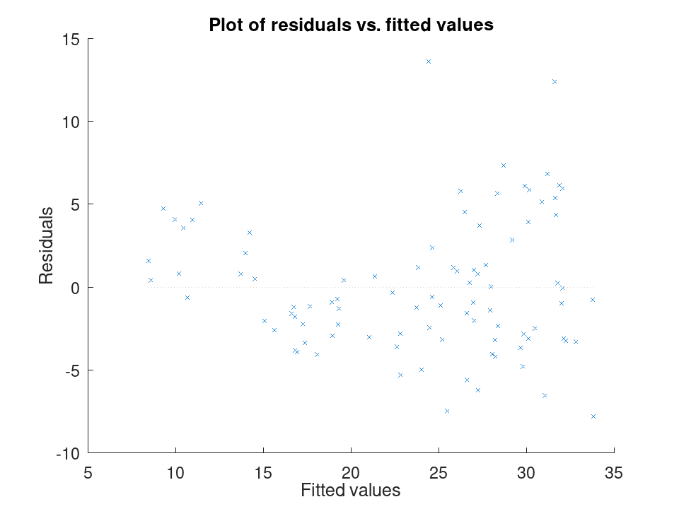
Spotting influential observations with Cook's distance. Sixteen houses are matched by size and age to a sale price, but one house was sold far above what its size and age would predict. After fitting the model, plotDiagnostics with the cookd option highlights that single observation as having outsized influence on the fit.
Size = [80; 95; 110; 120; 65; 140; 100; 130; 90; 150; 75; 105; ...
115; 85; 135; 125];
Age = [5; 10; 3; 8; 20; 2; 15; 6; 12; 1; 18; 9; 4; 14; 7; 11];
Price = [200; 230; 260; 280; 150; 320; 240; 300; 210; 340; 170; ...
250; 270; 190; 500; 290];
X = [Size, Age];
y = Price;
mdl = fitlm (X, y);
plotDiagnostics (mdl, 'cookd')
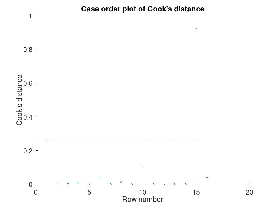
Comparing the size of each predictor's effect, alongside a hypothesis test on the model as a whole. We fit a mileage model on the carsmall data set using weight and horsepower. plotEffects draws each coefficient's estimate with its confidence interval side by side, and coefTest checks whether weight's effect is significantly different from horsepower's.
load carsmall X = [Weight, Horsepower]; y = MPG; mdl = fitlm (X, y);
Visualize the relative size of each predictor's effect.
plotEffects (mdl)
Test whether the two coefficients differ significantly.
H = [0 1 -1]; [p, F, r] = coefTest (mdl, H)
p = 0.073643 F = 3.2759 r = 1
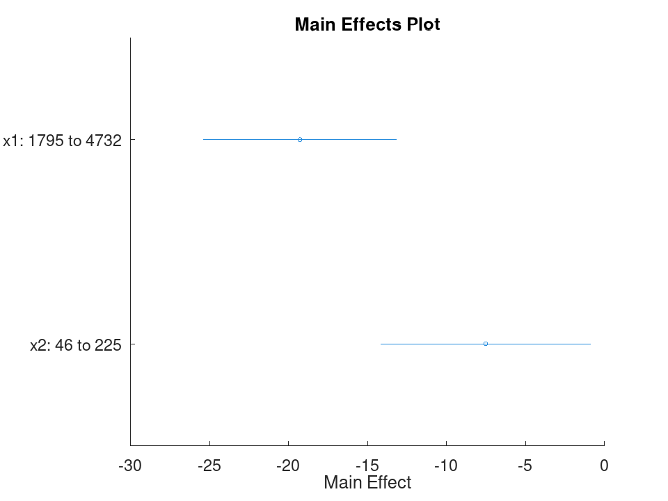
LinearModel: tbl = anova (mdl)
LinearModel: tbl = anova (mdl, anovatype)
LinearModel: tbl = anova (mdl, "components", sstype)
anova (mdl) returns a table tbl with component
ANOVA statistics for every term in mdl except the constant
term, computed with hierarchical ("h") sums of squares. Each
row gives SumSq, DF, MeanSq, F, and
pValue for the corresponding term; the trailing Error
row gives SumSq = mdl.SSE, DF = mdl.DFE,
MeanSq = mdl.MSE, and NaN for F and
pValue.
MATLAB reports F = 1 and pValue = 0.5 on that
Error row instead. Those are not results: the row’s F
is its own MeanSq divided by itself, so it is 1 for every
data set, and the pValue follows. MATLAB does not use them
consistently either, reporting NaN for the same quantity on the
Residual row of its summary table. This implementation reports
NaN in both places. Every other value in both tables agrees
with MATLAB.
anova (mdl, anovatype) selects
"components" (default) or "summary". For
"summary", tbl always contains rows Total,
Model, and Residual, and additionally . Linear
and . Nonlinear whenever mdl contains an interaction
term or a continuous term of degree greater than 1. Total
reports mdl.SST with DF = NumObservations - 1;
Model reports mdl.SSR with DF =
NumCoefficients - HasIntercept; Residual reports
mdl.SSE with DF = mdl.DFE. Whenever the
data contains two or more observations sharing identical predictor
values, tbl additionally contains . Lack of fit and
. Pure error, splitting Residual into the part
explained by replicated observations and the remainder.
anova (mdl, selects
the sum of squares used for the component table: "components", sstype)1 (sequential,
reduction from adding each term in formula order), 2 (reduction
from adding the term to a model containing every term that does not
contain it), "h" (default; as Type 2, but a higher-degree
term in the same continuous variable, such as a squared term, is also
treated as containing the lower-degree term), or 3 (reduction
from adding the term to a model containing every other term, with
categorical predictors recoded using sum-to-zero deviation contrasts
instead of mdl’s reference-level coding). Because Type 3 uses a
different coding, its Error row can differ from mdl.SSE
and mdl.DFE when mdl is missing a lower-order relative of
one of its terms (e.g. an interaction without one of its main
effects, or a categorical predictor fit without an intercept).
Simple linear regression with a single predictor. Ten runners record their weekly training distance and their finish time in a 10k race. We fit a straight line through this data and look at the fitted coefficients, then use predict to estimate the finish time for a runner who trains a distance not in the sample.
Distance = [10; 15; 20; 25; 30; 35; 40; 45; 50; 55]; Time = [58; 55; 52; 50; 47; 45; 43; 41; 40; 38]; X = Distance; y = Time;
Fit the model and inspect the estimated slope and intercept.
mdl = fitlm (X, y)
mdl =
Linear regression model:
y ~ 1 + x1
Estimated Coefficients:
2x4 table
Estimate SE tStat pValue
________ _________ ________ ___________
(Intercept) 61.2 0.654588 93.494 1.91213e-13
x1 -0.44 0.0184226 -23.8836 1.00609e-08
Number of observations: 10, Error degrees of freedom: 8
Root Mean Squared Error: 0.83666
R-squared: 0.986169, Adjusted R-Squared: 0.984441
F-statistic vs. constant model: 570.429, p-value = 1.00609e-08
Predict the finish time for a runner training 32 km per week.
ypred = predict (mdl, 32)
ypred = 47.120
Multiple linear regression with two predictors, followed by a confidence interval on the coefficients. Thirteen coffee shops report their weekly foot traffic and the number of items on their menu, along with weekly revenue. We fit a model with both predictors, then use coefCI to see how precisely each coefficient is estimated.
Traffic = [120; 150; 90; 200; 175; 60; 220; 140; 100; 190; 80; 210; 130];
MenuSize = [8; 12; 6; 15; 10; 5; 18; 9; 7; 14; 6; 16; 11];
Revenue = [1450; 1820; 1010; 2400; 2050; 700; 2650; 1700; 1150; ...
2300; 900; 2500; 1600];
X = [Traffic, MenuSize];
y = Revenue;
Fit the model with both predictors together.
mdl = fitlm (X, y)
mdl =
Linear regression model:
y ~ 1 + x1 + x2
Estimated Coefficients:
3x4 table
Estimate SE tStat pValue
________ ________ ________ ___________
(Intercept) -47.0932 27.3456 -1.72215 0.115771
x1 11.4079 0.616078 18.517 4.55169e-09
x2 11.4344 7.68384 1.48811 0.167562
Number of observations: 13, Error degrees of freedom: 10
Root Mean Squared Error: 32.4551
R-squared: 0.997901, Adjusted R-Squared: 0.997482
F-statistic vs. constant model: 2377.53, p-value = 4.07061e-14
Check how tight the 95% confidence interval is on each coefficient.
ci = coefCI (mdl)
ci =
-108.0231 13.8366
10.0352 12.7806
-5.6862 28.5551
Growing a model with addTerms and predicting with the richer model. We model fuel economy from the carsmall data set using weight and horsepower as main effects only. addTerms then brings in the weight-horsepower interaction without needing to refit by hand, and predict shows how the estimate for a new car changes once that interaction is included.
load carsmall X = [Weight, Horsepower]; y = MPG;
Fit the additive model first.
mdl = fitlm (X, y);
Add the interaction between weight and horsepower.
mdl2 = addTerms (mdl, 'x1:x2');
Compare predictions from both models for the same new car.
Xnew = [3200, 120]; ypred1 = predict (mdl, Xnew)
ypred1 = 21.719
ypred2 = predict (mdl2, Xnew)
ypred2 = 20.416
Simplifying a model with removeTerms and comparing fit quality. We fit the full Hald cement model with all four ingredients, then use removeTerms to drop the weakest predictor and refit automatically. Comparing SSE before and after shows how little explanatory power that ingredient was actually contributing.
load hald X = ingredients; y = heat;
Fit the model with all four ingredients.
mdl = fitlm (X, y);
Drop the third ingredient and refit on the same data.
mdl2 = removeTerms (mdl, 'x3');
Compare how much the error sum of squares changed.
sse_full = mdl.SSE
sse_full = 47.864
sse_reduced = mdl2.SSE
sse_reduced = 47.973
Testing a linear hypothesis and checking residual autocorrelation. Twelve patients are given a drug at different doses over different treatment durations, and a recovery score is recorded. coefTest checks whether the dose and duration coefficients are actually equal, and dwtest separately checks whether the residuals still carry a leftover pattern the model failed to capture.
Dose = [10; 15; 20; 25; 30; 35; 12; 18; 22; 28; 32; 38]; Duration = [5; 7; 9; 11; 13; 15; 6; 8; 10; 12; 14; 16]; Recovery = [42; 48; 55; 60; 68; 74; 45; 52; 58; 65; 71; 78]; X = [Dose, Duration]; y = Recovery; mdl = fitlm (X, y);
Test H0: the Dose and Duration coefficients are equal.
H = [0 1 -1]; [p, F, r] = coefTest (mdl, H)
p = 0.3535 F = 0.9571 r = 1
Check for autocorrelation left over in the residuals.
[pdw, dw] = dwtest (mdl)
pdw = 0.3658 dw = 2.4432
Checking residuals against fitted values. We fit a mileage model on the carsmall data set using weight and horsepower, then plot the raw residuals against the fitted values. A pattern in this plot, rather than a random scatter, would suggest the linear model is missing some curvature in the relationship.
load carsmall X = [Weight, Horsepower]; y = MPG; mdl = fitlm (X, y); plotResiduals (mdl, 'fitted')
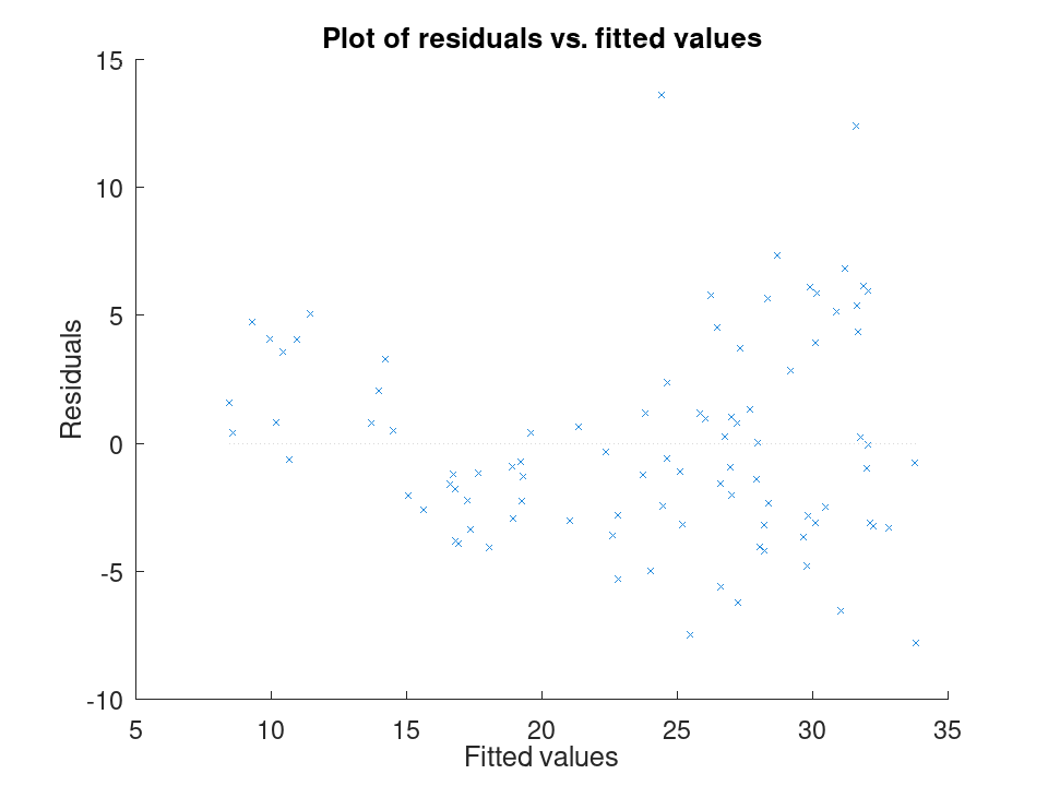
Spotting influential observations with Cook's distance. Sixteen houses are matched by size and age to a sale price, but one house was sold far above what its size and age would predict. After fitting the model, plotDiagnostics with the cookd option highlights that single observation as having outsized influence on the fit.
Size = [80; 95; 110; 120; 65; 140; 100; 130; 90; 150; 75; 105; ...
115; 85; 135; 125];
Age = [5; 10; 3; 8; 20; 2; 15; 6; 12; 1; 18; 9; 4; 14; 7; 11];
Price = [200; 230; 260; 280; 150; 320; 240; 300; 210; 340; 170; ...
250; 270; 190; 500; 290];
X = [Size, Age];
y = Price;
mdl = fitlm (X, y);
plotDiagnostics (mdl, 'cookd')
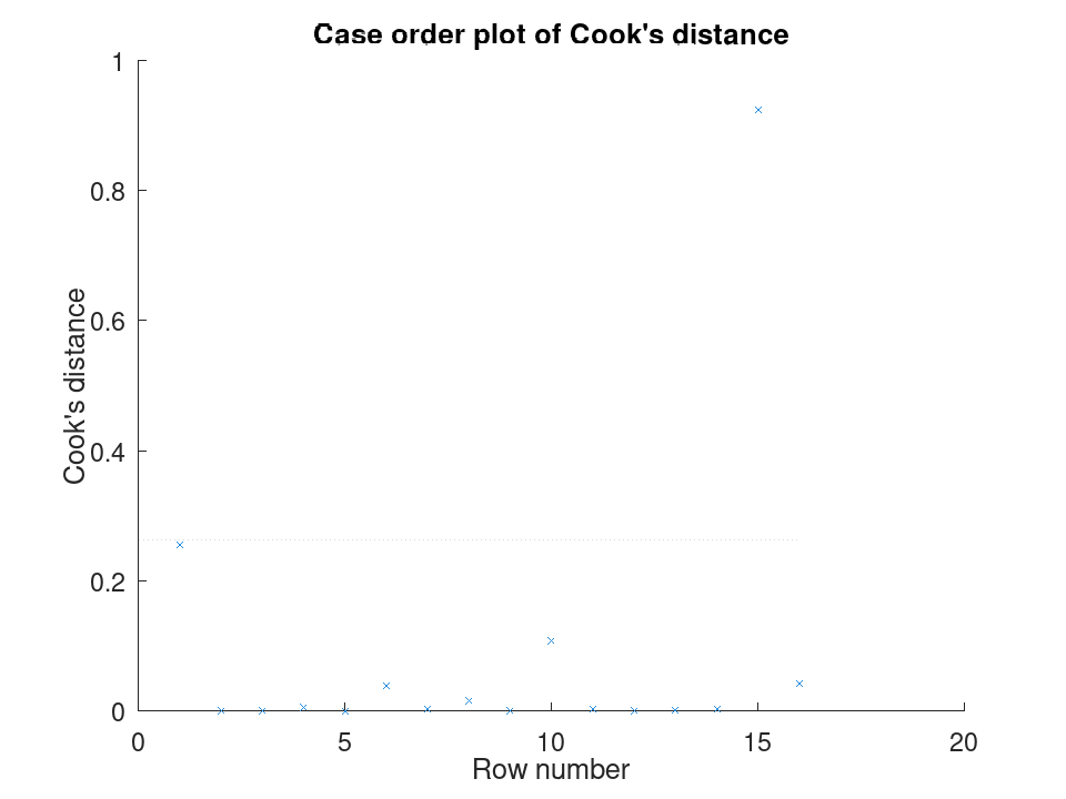
Comparing the size of each predictor's effect, alongside a hypothesis test on the model as a whole. We fit a mileage model on the carsmall data set using weight and horsepower. plotEffects draws each coefficient's estimate with its confidence interval side by side, and coefTest checks whether weight's effect is significantly different from horsepower's.
load carsmall X = [Weight, Horsepower]; y = MPG; mdl = fitlm (X, y);
Visualize the relative size of each predictor's effect.
plotEffects (mdl)
Test whether the two coefficients differ significantly.
H = [0 1 -1]; [p, F, r] = coefTest (mdl, H)
p = 0.073643 F = 3.2759 r = 1
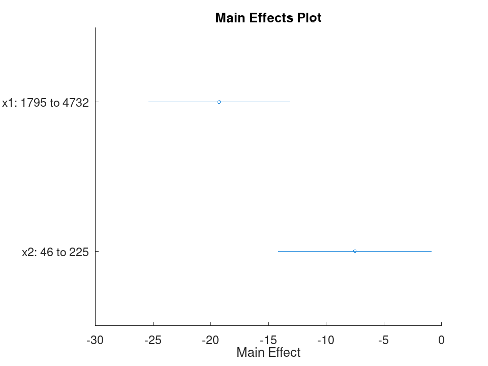
LinearModel: NewMdl = step (mdl)
LinearModel: NewMdl = step (mdl, Name, Value)
step examines whether adding or removing a single term from
mdl improves the fit, and returns the resulting model as
NewMdl. The original model mdl is never modified. Unlike
stepwiselm, step performs only one such improvement step
by default; pass 'NSteps' to allow more.
step accepts the same 'Criterion', 'PEnter',
'PRemove', 'NSteps', 'Verbose', 'Lower',
and 'Upper' Name-Value options as stepwiselm, with the
same defaults, except 'NSteps' defaults to 1 rather than
unlimited. mdl’s own predictors, weights, excluded observations,
and categorical variable settings are carried over automatically as
the starting point for the search.
step is not available for a model fitted with robust
regression.
See also: stepwiselm, LinearModel.addTerms, LinearModel.removeTerms
A single default step, improving a starting model by one term. Ten observations depend on study hours and hours of sleep. Starting from a model containing only x1, step examines whether adding or removing a single term improves the fit and, by default, takes at most one such step.
Hours = [1;2;3;4;5;6;7;8;9;10]; Sleep = [5;6;5;7;6;8;7;6;8;7]; Score = [50;54;56;62;64;70;71;73;79;78]; mdl0 = fitlm ([Hours, Sleep], Score, 'y ~ x1'); mdl0.CoefficientNames
ans =
1x2 cell array
{'(Intercept)'} {'x1'}
One improvement step, starting from x1 alone.
mdl1 = step (mdl0);
1. Adding x2, FStat = 25.5329, pValue = 0.001474845
mdl1.CoefficientNames
ans =
1x3 cell array
{'(Intercept)'} {'x1'} {'x2'}
Taking several steps at once with NSteps, and following the trace with Verbose. Reusing the same predictors, starting from a constant model this time, NSteps lets step keep improving the model over more than one call, up to the given upper bound.
Hours = [1;2;3;4;5;6;7;8;9;10]; Sleep = [5;6;5;7;6;8;7;6;8;7]; Score = [50;54;56;62;64;70;71;73;79;78]; mdl0 = fitlm ([Hours, Sleep], Score, 'y ~ 1');
Up to three steps, bounded above by the full interaction model.
mdl = step (mdl0, 'Upper', 'y ~ x1*x2', 'NSteps', 3, 'Verbose', 1);
1. Adding x1, FStat = 326.94, pValue = 8.985492e-08 2. Adding x2, FStat = 25.5329, pValue = 0.001474845
mdl.CoefficientNames
ans =
1x3 cell array
{'(Intercept)'} {'x1'} {'x2'}
Starting from a constant model on the hald cement data set. Four chemical percentages in cement (ingredients) are used to predict heat given off while hardening (heat). Starting from an intercept-only model, step adds the two most useful ingredients over several steps.
load hald mdl0 = fitlm (ingredients, heat, 'y ~ 1');
Up to four steps, bounded above by the additive model.
mdl = step (mdl0, 'Upper', 'linear', 'NSteps', 4, 'Verbose', 1);
1. Adding x4, FStat = 22.7985, pValue = 0.0005762318 2. Adding x1, FStat = 108.224, pValue = 1.105281e-06
mdl.CoefficientNames
ans =
1x3 cell array
{'(Intercept)'} {'x1'} {'x4'}
Examples
Distance = [10; 15; 20; 25; 30; 35; 40; 45; 50; 55]; Time = [58; 55; 52; 50; 47; 45; 43; 41; 40; 38]; X = Distance; y = Time;
Fit the model and inspect the estimated slope and intercept.
mdl = fitlm (X, y)
mdl =
Linear regression model:
y ~ 1 + x1
Estimated Coefficients:
2x4 table
Estimate SE tStat pValue
________ _________ ________ ___________
(Intercept) 61.2 0.654588 93.494 1.91213e-13
x1 -0.44 0.0184226 -23.8836 1.00609e-08
Number of observations: 10, Error degrees of freedom: 8
Root Mean Squared Error: 0.83666
R-squared: 0.986169, Adjusted R-Squared: 0.984441
F-statistic vs. constant model: 570.429, p-value = 1.00609e-08
Predict the finish time for a runner training 32 km per week.
ypred = predict (mdl, 32)
ypred = 47.120
Traffic = [120; 150; 90; 200; 175; 60; 220; 140; 100; 190; 80; 210; 130];
MenuSize = [8; 12; 6; 15; 10; 5; 18; 9; 7; 14; 6; 16; 11];
Revenue = [1450; 1820; 1010; 2400; 2050; 700; 2650; 1700; 1150; ...
2300; 900; 2500; 1600];
X = [Traffic, MenuSize];
y = Revenue;
Fit the model with both predictors together.
mdl = fitlm (X, y)
mdl =
Linear regression model:
y ~ 1 + x1 + x2
Estimated Coefficients:
3x4 table
Estimate SE tStat pValue
________ ________ ________ ___________
(Intercept) -47.0932 27.3456 -1.72215 0.115771
x1 11.4079 0.616078 18.517 4.55169e-09
x2 11.4344 7.68384 1.48811 0.167562
Number of observations: 13, Error degrees of freedom: 10
Root Mean Squared Error: 32.4551
R-squared: 0.997901, Adjusted R-Squared: 0.997482
F-statistic vs. constant model: 2377.53, p-value = 4.07061e-14
Check how tight the 95% confidence interval is on each coefficient.
ci = coefCI (mdl)
ci =
-108.0231 13.8366
10.0352 12.7806
-5.6862 28.5551
load carsmall X = [Weight, Horsepower]; y = MPG;
Fit the additive model first.
mdl = fitlm (X, y);
Add the interaction between weight and horsepower.
mdl2 = addTerms (mdl, 'x1:x2');
Compare predictions from both models for the same new car.
Xnew = [3200, 120]; ypred1 = predict (mdl, Xnew)
ypred1 = 21.719
ypred2 = predict (mdl2, Xnew)
ypred2 = 20.416
load hald X = ingredients; y = heat;
Fit the model with all four ingredients.
mdl = fitlm (X, y);
Drop the third ingredient and refit on the same data.
mdl2 = removeTerms (mdl, 'x3');
Compare how much the error sum of squares changed.
sse_full = mdl.SSE
sse_full = 47.864
sse_reduced = mdl2.SSE
sse_reduced = 47.973
Dose = [10; 15; 20; 25; 30; 35; 12; 18; 22; 28; 32; 38]; Duration = [5; 7; 9; 11; 13; 15; 6; 8; 10; 12; 14; 16]; Recovery = [42; 48; 55; 60; 68; 74; 45; 52; 58; 65; 71; 78]; X = [Dose, Duration]; y = Recovery; mdl = fitlm (X, y);
Test H0: the Dose and Duration coefficients are equal.
H = [0 1 -1]; [p, F, r] = coefTest (mdl, H)
p = 0.3535 F = 0.9571 r = 1
Check for autocorrelation left over in the residuals.
[pdw, dw] = dwtest (mdl)
pdw = 0.3658 dw = 2.4432
load carsmall X = [Weight, Horsepower]; y = MPG; mdl = fitlm (X, y); plotResiduals (mdl, 'fitted')
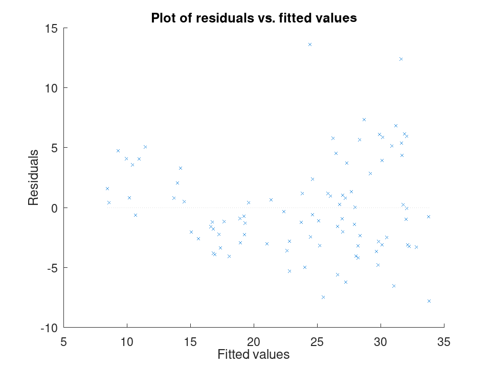
Size = [80; 95; 110; 120; 65; 140; 100; 130; 90; 150; 75; 105; ...
115; 85; 135; 125];
Age = [5; 10; 3; 8; 20; 2; 15; 6; 12; 1; 18; 9; 4; 14; 7; 11];
Price = [200; 230; 260; 280; 150; 320; 240; 300; 210; 340; 170; ...
250; 270; 190; 500; 290];
X = [Size, Age];
y = Price;
mdl = fitlm (X, y);
plotDiagnostics (mdl, 'cookd')
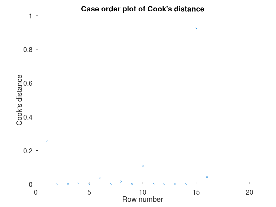
load carsmall X = [Weight, Horsepower]; y = MPG; mdl = fitlm (X, y);
Visualize the relative size of each predictor's effect.
plotEffects (mdl)
Test whether the two coefficients differ significantly.
H = [0 1 -1]; [p, F, r] = coefTest (mdl, H)
p = 0.073643 F = 3.2759 r = 1