Statistics: anova

Class Definition: `anova`

statistics: anova

Object-oriented interface for analysis of variance.

The anova class provides a MATLAB-compatible object interface for analysis of variance. It stores factors, response data, model specification, and fitted results in one object. The class chooses the narrowest compatible backend, delegates the numeric computation to the existing ANOVA functions, and exposes common follow-up operations such as stats, groupmeans, boxchart, plotComparisons, varianceComponent, and multcompare.

Models are fitted lazily. Methods that need fitted results call fit internally when necessary, so users may construct an object and immediately call inspection or post-hoc methods.

See also: anova1, anova2, anovan, multcompare

Source Code: anova

The anova class contains the following properties:

Numeric response vector (or matrix, for the one-way column form) used to fit the ANOVA model. This property is read-only.

Fit an ANOVA object and inspect component and summary statistics

 y = [1; 2; 3; 4; 5; 6; 10; 11; 12];
 g = [1; 1; 1; 2; 2; 2; 3; 3; 3];
 aov = anova (g, y, 'FactorNames', {'Treatment'});
 component = stats (aov)

component =
  3x5 table

                 SumOfSquares    DF    MeanSquares     F       pValue       
                 ____________    __    ___________    ___    ___________    

    Treatment             126     2             63     63    9.39144e-05    
    Error                   6     6              1    NaN            NaN    
    Total                 132     8            NaN    NaN            NaN

 summary_table = stats (aov, 'summary')

summary_table =
  4x5 table

                  SumOfSquares    DF    MeanSquares     F       pValue       
                  ____________    __    ___________    ___    ___________    

    Linear                 126     2             63     63    9.39144e-05    
    Regression             126     2             63     63    9.39144e-05    
    Error                    6     6              1    NaN            NaN    
    Total                  132     8           16.5    NaN            NaN

Estimate group means and perform post-hoc comparisons

 y = [1; 2; 3; 4; 5; 6; 10; 11; 12];
 g = [1; 1; 1; 2; 2; 2; 3; 3; 3];
 aov = anova (g, y, 'SumOfSquaresType', 'two');
 means = groupmeans (aov)

means =
  3x5 table

    Factor1    Mean      SE       MeanLower    MeanUpper    
    _______    ____    _______    _________    _________    

          1       2    0.57735     0.587275      3.41273    
          2       5    0.57735      3.58727      6.41273    
          3      11    0.57735      9.58727      12.4127

 comparisons = multcompare (aov, 'display', 'off')

comparisons =
  3x6 table

    Group1    Group2    MeanDifference    MeanDifferenceLower    MeanDifferenceUpper     pValue     
    ______    ______    ______________    ___________________    ___________________    ________    

         1         2                -3               -5.50561              -0.494388     0.02419    
         1         3                -9               -11.5056               -6.49439     8.9e-05    
         2         3                -6               -8.50561               -3.49439    0.000809

Plot multiple-comparison intervals

 y = [1; 2; 3; 4; 5; 6; 10; 11; 12];
 g = [1; 1; 1; 2; 2; 2; 3; 3; 3];
 aov = anova (g, y, 'SumOfSquaresType', 'two');
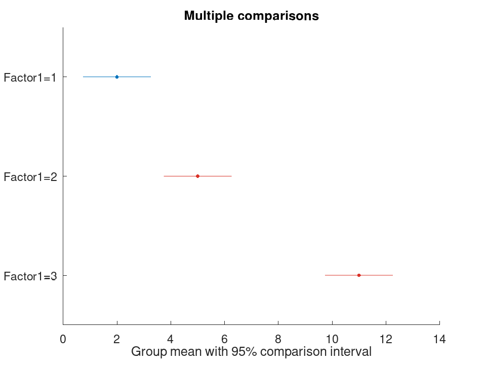
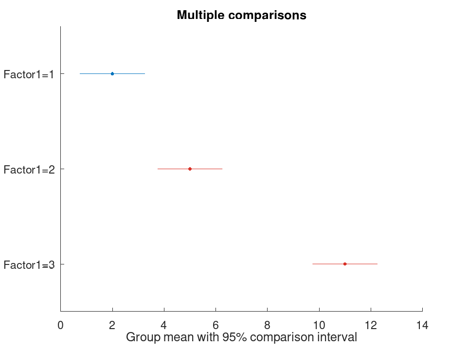
 plotComparisons (aov);

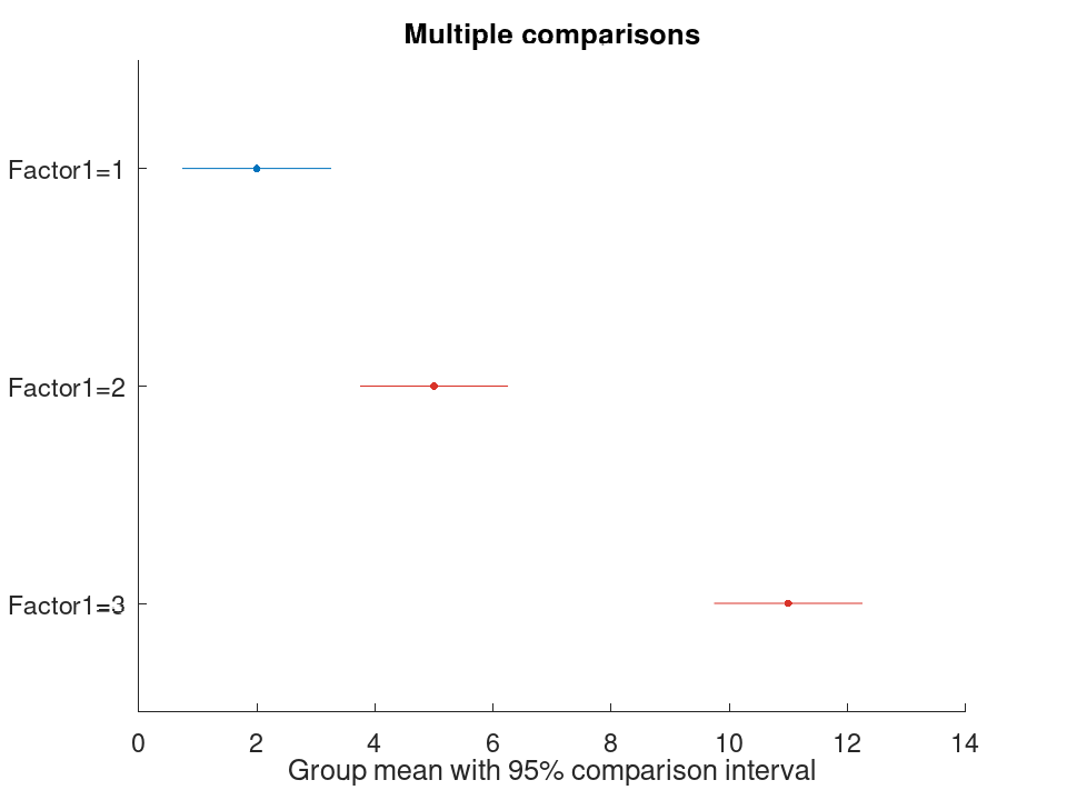
Table containing one variable for each factor used to fit the ANOVA model. This property is read-only.

Fit an ANOVA object and inspect component and summary statistics

 y = [1; 2; 3; 4; 5; 6; 10; 11; 12];
 g = [1; 1; 1; 2; 2; 2; 3; 3; 3];
 aov = anova (g, y, 'FactorNames', {'Treatment'});
 component = stats (aov)

component =
  3x5 table

                 SumOfSquares    DF    MeanSquares     F       pValue       
                 ____________    __    ___________    ___    ___________    

    Treatment             126     2             63     63    9.39144e-05    
    Error                   6     6              1    NaN            NaN    
    Total                 132     8            NaN    NaN            NaN

 summary_table = stats (aov, 'summary')

summary_table =
  4x5 table

                  SumOfSquares    DF    MeanSquares     F       pValue       
                  ____________    __    ___________    ___    ___________    

    Linear                 126     2             63     63    9.39144e-05    
    Regression             126     2             63     63    9.39144e-05    
    Error                    6     6              1    NaN            NaN    
    Total                  132     8           16.5    NaN            NaN

Estimate group means and perform post-hoc comparisons

 y = [1; 2; 3; 4; 5; 6; 10; 11; 12];
 g = [1; 1; 1; 2; 2; 2; 3; 3; 3];
 aov = anova (g, y, 'SumOfSquaresType', 'two');
 means = groupmeans (aov)

means =
  3x5 table

    Factor1    Mean      SE       MeanLower    MeanUpper    
    _______    ____    _______    _________    _________    

          1       2    0.57735     0.587275      3.41273    
          2       5    0.57735      3.58727      6.41273    
          3      11    0.57735      9.58727      12.4127

 comparisons = multcompare (aov, 'display', 'off')

comparisons =
  3x6 table

    Group1    Group2    MeanDifference    MeanDifferenceLower    MeanDifferenceUpper     pValue     
    ______    ______    ______________    ___________________    ___________________    ________    

         1         2                -3               -5.50187              -0.498133     0.02412    
         1         3                -9               -11.5019               -6.49813       9e-05    
         2         3                -6               -8.50187               -3.49813    0.000796

Plot multiple-comparison intervals

 y = [1; 2; 3; 4; 5; 6; 10; 11; 12];
 g = [1; 1; 1; 2; 2; 2; 3; 3; 3];
 aov = anova (g, y, 'SumOfSquaresType', 'two');
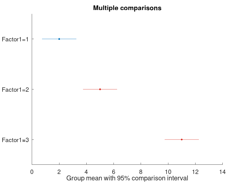
 plotComparisons (aov);

Read-only structural formula value with response, predictor, term, nesting, and linear-predictor fields matching MATLAB’s formula object.

Fit an ANOVA object and inspect component and summary statistics

 y = [1; 2; 3; 4; 5; 6; 10; 11; 12];
 g = [1; 1; 1; 2; 2; 2; 3; 3; 3];
 aov = anova (g, y, 'FactorNames', {'Treatment'});
 component = stats (aov)

component =
  3x5 table

                 SumOfSquares    DF    MeanSquares     F       pValue       
                 ____________    __    ___________    ___    ___________    

    Treatment             126     2             63     63    9.39144e-05    
    Error                   6     6              1    NaN            NaN    
    Total                 132     8            NaN    NaN            NaN

 summary_table = stats (aov, 'summary')

summary_table =
  4x5 table

                  SumOfSquares    DF    MeanSquares     F       pValue       
                  ____________    __    ___________    ___    ___________    

    Linear                 126     2             63     63    9.39144e-05    
    Regression             126     2             63     63    9.39144e-05    
    Error                    6     6              1    NaN            NaN    
    Total                  132     8           16.5    NaN            NaN

Estimate group means and perform post-hoc comparisons

 y = [1; 2; 3; 4; 5; 6; 10; 11; 12];
 g = [1; 1; 1; 2; 2; 2; 3; 3; 3];
 aov = anova (g, y, 'SumOfSquaresType', 'two');
 means = groupmeans (aov)

means =
  3x5 table

    Factor1    Mean      SE       MeanLower    MeanUpper    
    _______    ____    _______    _________    _________    

          1       2    0.57735     0.587275      3.41273    
          2       5    0.57735      3.58727      6.41273    
          3      11    0.57735      9.58727      12.4127

 comparisons = multcompare (aov, 'display', 'off')

comparisons =
  3x6 table

    Group1    Group2    MeanDifference    MeanDifferenceLower    MeanDifferenceUpper     pValue     
    ______    ______    ______________    ___________________    ___________________    ________    

         1         2                -3               -5.50574              -0.494264    0.024268    
         1         3                -9               -11.5057               -6.49426     9.6e-05    
         2         3                -6               -8.50574               -3.49426    0.000823

Plot multiple-comparison intervals

 y = [1; 2; 3; 4; 5; 6; 10; 11; 12];
 g = [1; 1; 1; 2; 2; 2; 3; 3; 3];
 aov = anova (g, y, 'SumOfSquaresType', 'two');
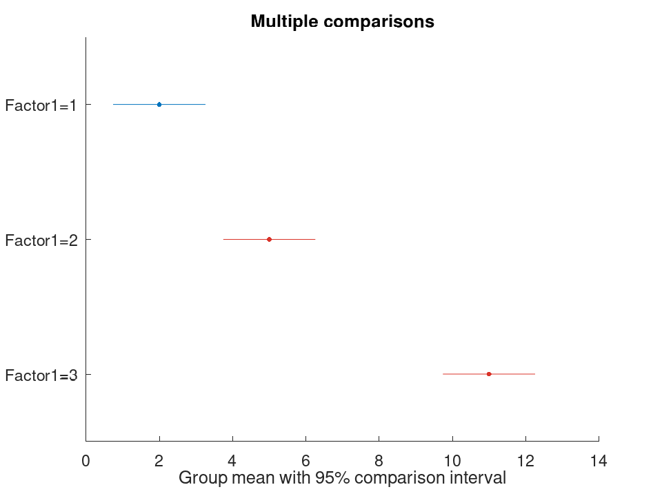
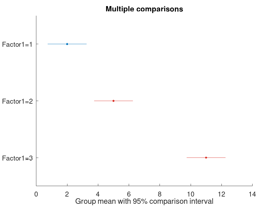
 plotComparisons (aov);

String row vector containing the factor names used by the fitted ANOVA model. This property is read-only.

Fit an ANOVA object and inspect component and summary statistics

 y = [1; 2; 3; 4; 5; 6; 10; 11; 12];
 g = [1; 1; 1; 2; 2; 2; 3; 3; 3];
 aov = anova (g, y, 'FactorNames', {'Treatment'});
 component = stats (aov)

component =
  3x5 table

                 SumOfSquares    DF    MeanSquares     F       pValue       
                 ____________    __    ___________    ___    ___________    

    Treatment             126     2             63     63    9.39144e-05    
    Error                   6     6              1    NaN            NaN    
    Total                 132     8            NaN    NaN            NaN

 summary_table = stats (aov, 'summary')

summary_table =
  4x5 table

                  SumOfSquares    DF    MeanSquares     F       pValue       
                  ____________    __    ___________    ___    ___________    

    Linear                 126     2             63     63    9.39144e-05    
    Regression             126     2             63     63    9.39144e-05    
    Error                    6     6              1    NaN            NaN    
    Total                  132     8           16.5    NaN            NaN

Estimate group means and perform post-hoc comparisons

 y = [1; 2; 3; 4; 5; 6; 10; 11; 12];
 g = [1; 1; 1; 2; 2; 2; 3; 3; 3];
 aov = anova (g, y, 'SumOfSquaresType', 'two');
 means = groupmeans (aov)

means =
  3x5 table

    Factor1    Mean      SE       MeanLower    MeanUpper    
    _______    ____    _______    _________    _________    

          1       2    0.57735     0.587275      3.41273    
          2       5    0.57735      3.58727      6.41273    
          3      11    0.57735      9.58727      12.4127

 comparisons = multcompare (aov, 'display', 'off')

comparisons =
  3x6 table

    Group1    Group2    MeanDifference    MeanDifferenceLower    MeanDifferenceUpper     pValue     
    ______    ______    ______________    ___________________    ___________________    ________    

         1         2                -3               -5.50924              -0.490758    0.024039    
         1         3                -9               -11.5092               -6.49076     7.9e-05    
         2         3                -6               -8.50924               -3.49076      0.0008

Plot multiple-comparison intervals

 y = [1; 2; 3; 4; 5; 6; 10; 11; 12];
 g = [1; 1; 1; 2; 2; 2; 3; 3; 3];
 aov = anova (g, y, 'SumOfSquaresType', 'two');
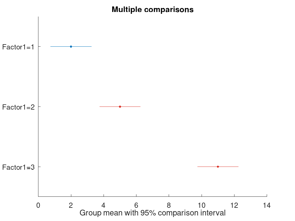
 plotComparisons (aov);

Cell array of character vectors naming the model coefficients when the selected backend exposes them, otherwise an empty cell array. This property is read-only.

Fit an ANOVA object and inspect component and summary statistics

 y = [1; 2; 3; 4; 5; 6; 10; 11; 12];
 g = [1; 1; 1; 2; 2; 2; 3; 3; 3];
 aov = anova (g, y, 'FactorNames', {'Treatment'});
 component = stats (aov)

component =
  3x5 table

                 SumOfSquares    DF    MeanSquares     F       pValue       
                 ____________    __    ___________    ___    ___________    

    Treatment             126     2             63     63    9.39144e-05    
    Error                   6     6              1    NaN            NaN    
    Total                 132     8            NaN    NaN            NaN

 summary_table = stats (aov, 'summary')

summary_table =
  4x5 table

                  SumOfSquares    DF    MeanSquares     F       pValue       
                  ____________    __    ___________    ___    ___________    

    Linear                 126     2             63     63    9.39144e-05    
    Regression             126     2             63     63    9.39144e-05    
    Error                    6     6              1    NaN            NaN    
    Total                  132     8           16.5    NaN            NaN

Estimate group means and perform post-hoc comparisons

 y = [1; 2; 3; 4; 5; 6; 10; 11; 12];
 g = [1; 1; 1; 2; 2; 2; 3; 3; 3];
 aov = anova (g, y, 'SumOfSquaresType', 'two');
 means = groupmeans (aov)

means =
  3x5 table

    Factor1    Mean      SE       MeanLower    MeanUpper    
    _______    ____    _______    _________    _________    

          1       2    0.57735     0.587275      3.41273    
          2       5    0.57735      3.58727      6.41273    
          3      11    0.57735      9.58727      12.4127

 comparisons = multcompare (aov, 'display', 'off')

comparisons =
  3x6 table

    Group1    Group2    MeanDifference    MeanDifferenceLower    MeanDifferenceUpper     pValue     
    ______    ______    ______________    ___________________    ___________________    ________    

         1         2                -3               -5.50832              -0.491681    0.024343    
         1         3                -9               -11.5083               -6.49168       9e-05    
         2         3                -6               -8.50832               -3.49168     0.00081

Plot multiple-comparison intervals

 y = [1; 2; 3; 4; 5; 6; 10; 11; 12];
 g = [1; 1; 1; 2; 2; 2; 3; 3; 3];
 aov = anova (g, y, 'SumOfSquaresType', 'two');
 plotComparisons (aov);

String scalar selecting "one", "two", 'three', or 'hierarchical' sums of squares. This property is read-only.

Fit an ANOVA object and inspect component and summary statistics

 y = [1; 2; 3; 4; 5; 6; 10; 11; 12];
 g = [1; 1; 1; 2; 2; 2; 3; 3; 3];
 aov = anova (g, y, 'FactorNames', {'Treatment'});
 component = stats (aov)

component =
  3x5 table

                 SumOfSquares    DF    MeanSquares     F       pValue       
                 ____________    __    ___________    ___    ___________    

    Treatment             126     2             63     63    9.39144e-05    
    Error                   6     6              1    NaN            NaN    
    Total                 132     8            NaN    NaN            NaN

 summary_table = stats (aov, 'summary')

summary_table =
  4x5 table

                  SumOfSquares    DF    MeanSquares     F       pValue       
                  ____________    __    ___________    ___    ___________    

    Linear                 126     2             63     63    9.39144e-05    
    Regression             126     2             63     63    9.39144e-05    
    Error                    6     6              1    NaN            NaN    
    Total                  132     8           16.5    NaN            NaN

Estimate group means and perform post-hoc comparisons

 y = [1; 2; 3; 4; 5; 6; 10; 11; 12];
 g = [1; 1; 1; 2; 2; 2; 3; 3; 3];
 aov = anova (g, y, 'SumOfSquaresType', 'two');
 means = groupmeans (aov)

means =
  3x5 table

    Factor1    Mean      SE       MeanLower    MeanUpper    
    _______    ____    _______    _________    _________    

          1       2    0.57735     0.587275      3.41273    
          2       5    0.57735      3.58727      6.41273    
          3      11    0.57735      9.58727      12.4127

 comparisons = multcompare (aov, 'display', 'off')

comparisons =
  3x6 table

    Group1    Group2    MeanDifference    MeanDifferenceLower    MeanDifferenceUpper     pValue     
    ______    ______    ______________    ___________________    ___________________    ________    

         1         2                -3               -5.50578              -0.494217    0.024162    
         1         3                -9               -11.5058               -6.49422     9.6e-05    
         2         3                -6               -8.50578               -3.49422    0.000809

Plot multiple-comparison intervals

 y = [1; 2; 3; 4; 5; 6; 10; 11; 12];
 g = [1; 1; 1; 2; 2; 2; 3; 3; 3];
 aov = anova (g, y, 'SumOfSquaresType', 'two');
 plotComparisons (aov);

Positive integer indices of random factors. This property is read-only.

Fit an ANOVA object and inspect component and summary statistics

 y = [1; 2; 3; 4; 5; 6; 10; 11; 12];
 g = [1; 1; 1; 2; 2; 2; 3; 3; 3];
 aov = anova (g, y, 'FactorNames', {'Treatment'});
 component = stats (aov)

component =
  3x5 table

                 SumOfSquares    DF    MeanSquares     F       pValue       
                 ____________    __    ___________    ___    ___________    

    Treatment             126     2             63     63    9.39144e-05    
    Error                   6     6              1    NaN            NaN    
    Total                 132     8            NaN    NaN            NaN

 summary_table = stats (aov, 'summary')

summary_table =
  4x5 table

                  SumOfSquares    DF    MeanSquares     F       pValue       
                  ____________    __    ___________    ___    ___________    

    Linear                 126     2             63     63    9.39144e-05    
    Regression             126     2             63     63    9.39144e-05    
    Error                    6     6              1    NaN            NaN    
    Total                  132     8           16.5    NaN            NaN

Estimate group means and perform post-hoc comparisons

 y = [1; 2; 3; 4; 5; 6; 10; 11; 12];
 g = [1; 1; 1; 2; 2; 2; 3; 3; 3];
 aov = anova (g, y, 'SumOfSquaresType', 'two');
 means = groupmeans (aov)

means =
  3x5 table

    Factor1    Mean      SE       MeanLower    MeanUpper    
    _______    ____    _______    _________    _________    

          1       2    0.57735     0.587275      3.41273    
          2       5    0.57735      3.58727      6.41273    
          3      11    0.57735      9.58727      12.4127

 comparisons = multcompare (aov, 'display', 'off')

comparisons =
  3x6 table

    Group1    Group2    MeanDifference    MeanDifferenceLower    MeanDifferenceUpper     pValue     
    ______    ______    ______________    ___________________    ___________________    ________    

         1         2                -3               -5.50021              -0.499794    0.024274    
         1         3                -9               -11.5002               -6.49979     8.7e-05    
         2         3                -6               -8.50021               -3.49979    0.000792

Plot multiple-comparison intervals

 y = [1; 2; 3; 4; 5; 6; 10; 11; 12];
 g = [1; 1; 1; 2; 2; 2; 3; 3; 3];
 aov = anova (g, y, 'SumOfSquaresType', 'two');
 plotComparisons (aov);

Positive integer indices of factors treated as categorical. This property is read-only.

Fit an ANOVA object and inspect component and summary statistics

 y = [1; 2; 3; 4; 5; 6; 10; 11; 12];
 g = [1; 1; 1; 2; 2; 2; 3; 3; 3];
 aov = anova (g, y, 'FactorNames', {'Treatment'});
 component = stats (aov)

component =
  3x5 table

                 SumOfSquares    DF    MeanSquares     F       pValue       
                 ____________    __    ___________    ___    ___________    

    Treatment             126     2             63     63    9.39144e-05    
    Error                   6     6              1    NaN            NaN    
    Total                 132     8            NaN    NaN            NaN

 summary_table = stats (aov, 'summary')

summary_table =
  4x5 table

                  SumOfSquares    DF    MeanSquares     F       pValue       
                  ____________    __    ___________    ___    ___________    

    Linear                 126     2             63     63    9.39144e-05    
    Regression             126     2             63     63    9.39144e-05    
    Error                    6     6              1    NaN            NaN    
    Total                  132     8           16.5    NaN            NaN

Estimate group means and perform post-hoc comparisons

 y = [1; 2; 3; 4; 5; 6; 10; 11; 12];
 g = [1; 1; 1; 2; 2; 2; 3; 3; 3];
 aov = anova (g, y, 'SumOfSquaresType', 'two');
 means = groupmeans (aov)

means =
  3x5 table

    Factor1    Mean      SE       MeanLower    MeanUpper    
    _______    ____    _______    _________    _________    

          1       2    0.57735     0.587275      3.41273    
          2       5    0.57735      3.58727      6.41273    
          3      11    0.57735      9.58727      12.4127

 comparisons = multcompare (aov, 'display', 'off')

comparisons =
  3x6 table

    Group1    Group2    MeanDifference    MeanDifferenceLower    MeanDifferenceUpper     pValue     
    ______    ______    ______________    ___________________    ___________________    ________    

         1         2                -3               -5.50598              -0.494017    0.024469    
         1         3                -9                -11.506               -6.49402     7.7e-05    
         2         3                -6               -8.50598               -3.49402    0.000796

Plot multiple-comparison intervals

 y = [1; 2; 3; 4; 5; 6; 10; 11; 12];
 g = [1; 1; 1; 2; 2; 2; 3; 3; 3];
 aov = anova (g, y, 'SumOfSquaresType', 'two');
 plotComparisons (aov);

Character vector used as the response name in formula display. This property is read-only.

Fit an ANOVA object and inspect component and summary statistics

 y = [1; 2; 3; 4; 5; 6; 10; 11; 12];
 g = [1; 1; 1; 2; 2; 2; 3; 3; 3];
 aov = anova (g, y, 'FactorNames', {'Treatment'});
 component = stats (aov)

component =
  3x5 table

                 SumOfSquares    DF    MeanSquares     F       pValue       
                 ____________    __    ___________    ___    ___________    

    Treatment             126     2             63     63    9.39144e-05    
    Error                   6     6              1    NaN            NaN    
    Total                 132     8            NaN    NaN            NaN

 summary_table = stats (aov, 'summary')

summary_table =
  4x5 table

                  SumOfSquares    DF    MeanSquares     F       pValue       
                  ____________    __    ___________    ___    ___________    

    Linear                 126     2             63     63    9.39144e-05    
    Regression             126     2             63     63    9.39144e-05    
    Error                    6     6              1    NaN            NaN    
    Total                  132     8           16.5    NaN            NaN

Estimate group means and perform post-hoc comparisons

 y = [1; 2; 3; 4; 5; 6; 10; 11; 12];
 g = [1; 1; 1; 2; 2; 2; 3; 3; 3];
 aov = anova (g, y, 'SumOfSquaresType', 'two');
 means = groupmeans (aov)

means =
  3x5 table

    Factor1    Mean      SE       MeanLower    MeanUpper    
    _______    ____    _______    _________    _________    

          1       2    0.57735     0.587275      3.41273    
          2       5    0.57735      3.58727      6.41273    
          3      11    0.57735      9.58727      12.4127

 comparisons = multcompare (aov, 'display', 'off')

comparisons =
  3x6 table

    Group1    Group2    MeanDifference    MeanDifferenceLower    MeanDifferenceUpper     pValue     
    ______    ______    ______________    ___________________    ___________________    ________    

         1         2                -3               -5.50806              -0.491942    0.024361    
         1         3                -9               -11.5081               -6.49194       7e-05    
         2         3                -6               -8.50806               -3.49194    0.000819

Plot multiple-comparison intervals

 y = [1; 2; 3; 4; 5; 6; 10; 11; 12];
 g = [1; 1; 1; 2; 2; 2; 3; 3; 3];
 aov = anova (g, y, 'SumOfSquaresType', 'two');
 plotComparisons (aov);

Scalar number of response observations used by the model. This property is read-only.

Fit an ANOVA object and inspect component and summary statistics

 y = [1; 2; 3; 4; 5; 6; 10; 11; 12];
 g = [1; 1; 1; 2; 2; 2; 3; 3; 3];
 aov = anova (g, y, 'FactorNames', {'Treatment'});
 component = stats (aov)

component =
  3x5 table

                 SumOfSquares    DF    MeanSquares     F       pValue       
                 ____________    __    ___________    ___    ___________    

    Treatment             126     2             63     63    9.39144e-05    
    Error                   6     6              1    NaN            NaN    
    Total                 132     8            NaN    NaN            NaN

 summary_table = stats (aov, 'summary')

summary_table =
  4x5 table

                  SumOfSquares    DF    MeanSquares     F       pValue       
                  ____________    __    ___________    ___    ___________    

    Linear                 126     2             63     63    9.39144e-05    
    Regression             126     2             63     63    9.39144e-05    
    Error                    6     6              1    NaN            NaN    
    Total                  132     8           16.5    NaN            NaN

Estimate group means and perform post-hoc comparisons

 y = [1; 2; 3; 4; 5; 6; 10; 11; 12];
 g = [1; 1; 1; 2; 2; 2; 3; 3; 3];
 aov = anova (g, y, 'SumOfSquaresType', 'two');
 means = groupmeans (aov)

means =
  3x5 table

    Factor1    Mean      SE       MeanLower    MeanUpper    
    _______    ____    _______    _________    _________    

          1       2    0.57735     0.587275      3.41273    
          2       5    0.57735      3.58727      6.41273    
          3      11    0.57735      9.58727      12.4127

 comparisons = multcompare (aov, 'display', 'off')

comparisons =
  3x6 table

    Group1    Group2    MeanDifference    MeanDifferenceLower    MeanDifferenceUpper     pValue     
    ______    ______    ______________    ___________________    ___________________    ________    

         1         2                -3               -5.50863              -0.491369    0.024226    
         1         3                -9               -11.5086               -6.49137     6.6e-05    
         2         3                -6               -8.50863               -3.49137    0.000797

Plot multiple-comparison intervals

 y = [1; 2; 3; 4; 5; 6; 10; 11; 12];
 g = [1; 1; 1; 2; 2; 2; 3; 3; 3];
 aov = anova (g, y, 'SumOfSquaresType', 'two');
 plotComparisons (aov);

Numeric vector of fitted coefficient estimates. This property is read-only.

Fit an ANOVA object and inspect component and summary statistics

 y = [1; 2; 3; 4; 5; 6; 10; 11; 12];
 g = [1; 1; 1; 2; 2; 2; 3; 3; 3];
 aov = anova (g, y, 'FactorNames', {'Treatment'});
 component = stats (aov)

component =
  3x5 table

                 SumOfSquares    DF    MeanSquares     F       pValue       
                 ____________    __    ___________    ___    ___________    

    Treatment             126     2             63     63    9.39144e-05    
    Error                   6     6              1    NaN            NaN    
    Total                 132     8            NaN    NaN            NaN

 summary_table = stats (aov, 'summary')

summary_table =
  4x5 table

                  SumOfSquares    DF    MeanSquares     F       pValue       
                  ____________    __    ___________    ___    ___________    

    Linear                 126     2             63     63    9.39144e-05    
    Regression             126     2             63     63    9.39144e-05    
    Error                    6     6              1    NaN            NaN    
    Total                  132     8           16.5    NaN            NaN

Estimate group means and perform post-hoc comparisons

 y = [1; 2; 3; 4; 5; 6; 10; 11; 12];
 g = [1; 1; 1; 2; 2; 2; 3; 3; 3];
 aov = anova (g, y, 'SumOfSquaresType', 'two');
 means = groupmeans (aov)

means =
  3x5 table

    Factor1    Mean      SE       MeanLower    MeanUpper    
    _______    ____    _______    _________    _________    

          1       2    0.57735     0.587275      3.41273    
          2       5    0.57735      3.58727      6.41273    
          3      11    0.57735      9.58727      12.4127

 comparisons = multcompare (aov, 'display', 'off')

comparisons =
  3x6 table

    Group1    Group2    MeanDifference    MeanDifferenceLower    MeanDifferenceUpper     pValue     
    ______    ______    ______________    ___________________    ___________________    ________    

         1         2                -3               -5.49904              -0.500961    0.024062    
         1         3                -9                -11.499               -6.50096       8e-05    
         2         3                -6               -8.49904               -3.50096    0.000838

Plot multiple-comparison intervals

 y = [1; 2; 3; 4; 5; 6; 10; 11; 12];
 g = [1; 1; 1; 2; 2; 2; 3; 3; 3];
 aov = anova (g, y, 'SumOfSquaresType', 'two');
 plotComparisons (aov);

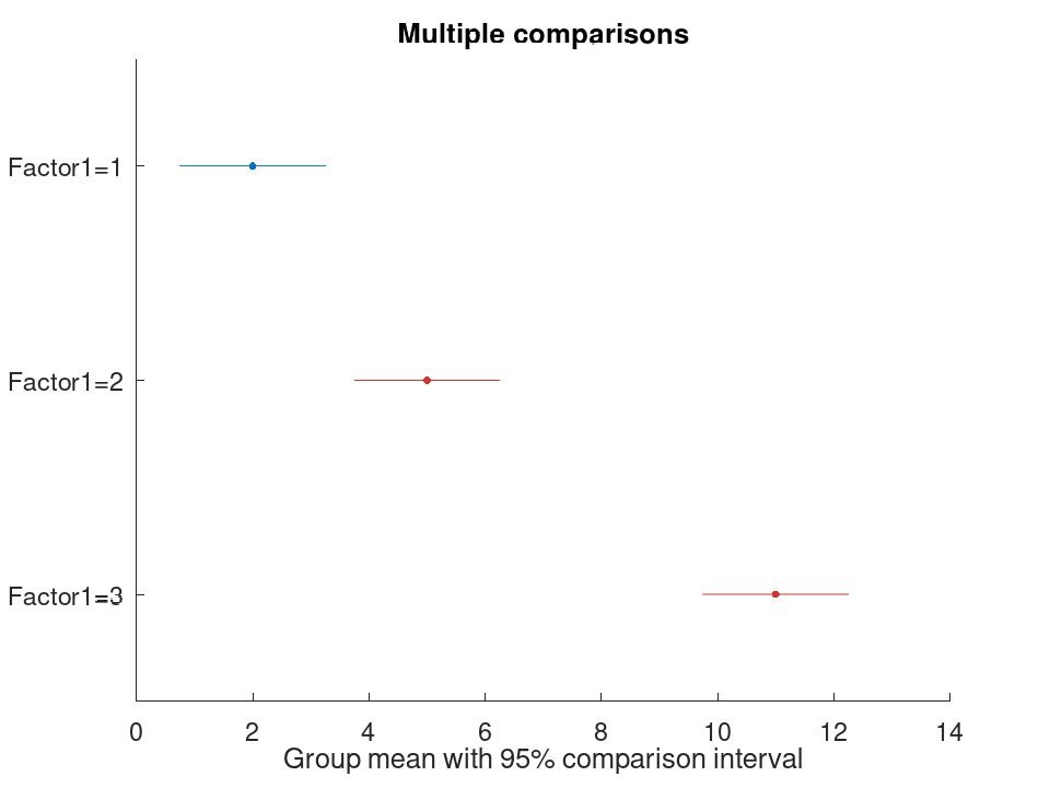
Table with variables Raw (observed minus fitted values) and Pearson (raw residuals scaled by the root mean squared error) when the selected backend exposes residuals, otherwise empty. This property is read-only.

Fit an ANOVA object and inspect component and summary statistics

 y = [1; 2; 3; 4; 5; 6; 10; 11; 12];
 g = [1; 1; 1; 2; 2; 2; 3; 3; 3];
 aov = anova (g, y, 'FactorNames', {'Treatment'});
 component = stats (aov)

component =
  3x5 table

                 SumOfSquares    DF    MeanSquares     F       pValue       
                 ____________    __    ___________    ___    ___________    

    Treatment             126     2             63     63    9.39144e-05    
    Error                   6     6              1    NaN            NaN    
    Total                 132     8            NaN    NaN            NaN

 summary_table = stats (aov, 'summary')

summary_table =
  4x5 table

                  SumOfSquares    DF    MeanSquares     F       pValue       
                  ____________    __    ___________    ___    ___________    

    Linear                 126     2             63     63    9.39144e-05    
    Regression             126     2             63     63    9.39144e-05    
    Error                    6     6              1    NaN            NaN    
    Total                  132     8           16.5    NaN            NaN

Estimate group means and perform post-hoc comparisons

 y = [1; 2; 3; 4; 5; 6; 10; 11; 12];
 g = [1; 1; 1; 2; 2; 2; 3; 3; 3];
 aov = anova (g, y, 'SumOfSquaresType', 'two');
 means = groupmeans (aov)

means =
  3x5 table

    Factor1    Mean      SE       MeanLower    MeanUpper    
    _______    ____    _______    _________    _________    

          1       2    0.57735     0.587275      3.41273    
          2       5    0.57735      3.58727      6.41273    
          3      11    0.57735      9.58727      12.4127

 comparisons = multcompare (aov, 'display', 'off')

comparisons =
  3x6 table

    Group1    Group2    MeanDifference    MeanDifferenceLower    MeanDifferenceUpper     pValue     
    ______    ______    ______________    ___________________    ___________________    ________    

         1         2                -3               -5.50718              -0.492821    0.024407    
         1         3                -9               -11.5072               -6.49282     8.8e-05    
         2         3                -6               -8.50718               -3.49282    0.000826

Plot multiple-comparison intervals

 y = [1; 2; 3; 4; 5; 6; 10; 11; 12];
 g = [1; 1; 1; 2; 2; 2; 3; 3; 3];
 aov = anova (g, y, 'SumOfSquaresType', 'two');
 plotComparisons (aov);

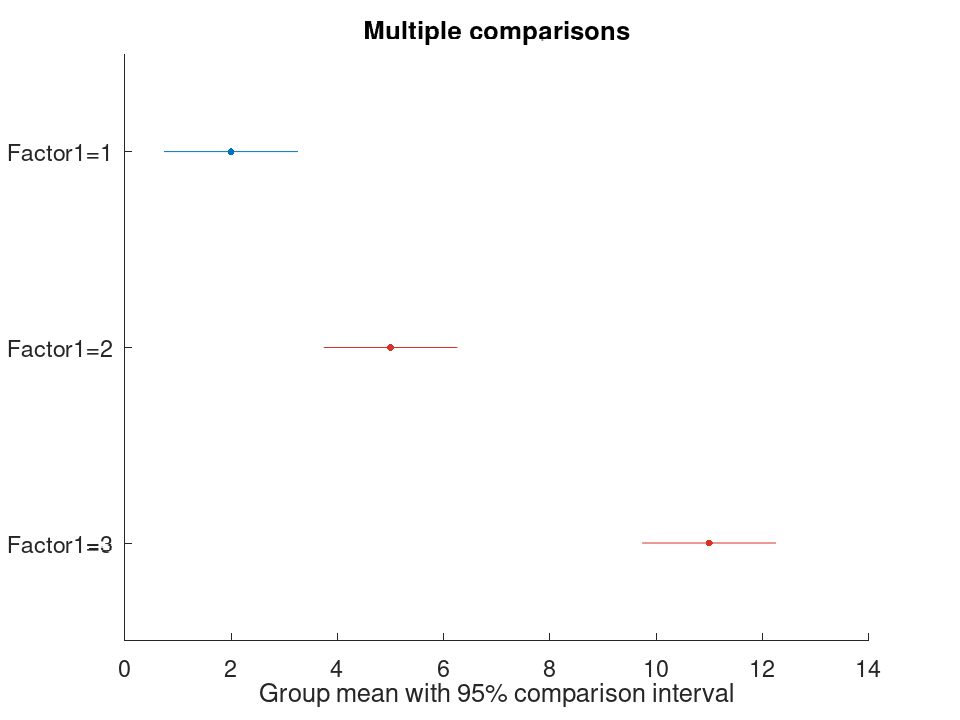
Table with variables MSE, RMSE, SSE, SSR, SST, RSquared, and AdjustedRSquared summarising the fitted model. This property is read-only.

Fit an ANOVA object and inspect component and summary statistics

 y = [1; 2; 3; 4; 5; 6; 10; 11; 12];
 g = [1; 1; 1; 2; 2; 2; 3; 3; 3];
 aov = anova (g, y, 'FactorNames', {'Treatment'});
 component = stats (aov)

component =
  3x5 table

                 SumOfSquares    DF    MeanSquares     F       pValue       
                 ____________    __    ___________    ___    ___________    

    Treatment             126     2             63     63    9.39144e-05    
    Error                   6     6              1    NaN            NaN    
    Total                 132     8            NaN    NaN            NaN

 summary_table = stats (aov, 'summary')

summary_table =
  4x5 table

                  SumOfSquares    DF    MeanSquares     F       pValue       
                  ____________    __    ___________    ___    ___________    

    Linear                 126     2             63     63    9.39144e-05    
    Regression             126     2             63     63    9.39144e-05    
    Error                    6     6              1    NaN            NaN    
    Total                  132     8           16.5    NaN            NaN

Estimate group means and perform post-hoc comparisons

 y = [1; 2; 3; 4; 5; 6; 10; 11; 12];
 g = [1; 1; 1; 2; 2; 2; 3; 3; 3];
 aov = anova (g, y, 'SumOfSquaresType', 'two');
 means = groupmeans (aov)

means =
  3x5 table

    Factor1    Mean      SE       MeanLower    MeanUpper    
    _______    ____    _______    _________    _________    

          1       2    0.57735     0.587275      3.41273    
          2       5    0.57735      3.58727      6.41273    
          3      11    0.57735      9.58727      12.4127

 comparisons = multcompare (aov, 'display', 'off')

comparisons =
  3x6 table

    Group1    Group2    MeanDifference    MeanDifferenceLower    MeanDifferenceUpper     pValue     
    ______    ______    ______________    ___________________    ___________________    ________    

         1         2                -3               -5.50702               -0.49298    0.024248    
         1         3                -9                -11.507               -6.49298     6.3e-05    
         2         3                -6               -8.50702               -3.49298    0.000789

Plot multiple-comparison intervals

 y = [1; 2; 3; 4; 5; 6; 10; 11; 12];
 g = [1; 1; 1; 2; 2; 2; 3; 3; 3];
 aov = anova (g, y, 'SumOfSquaresType', 'two');
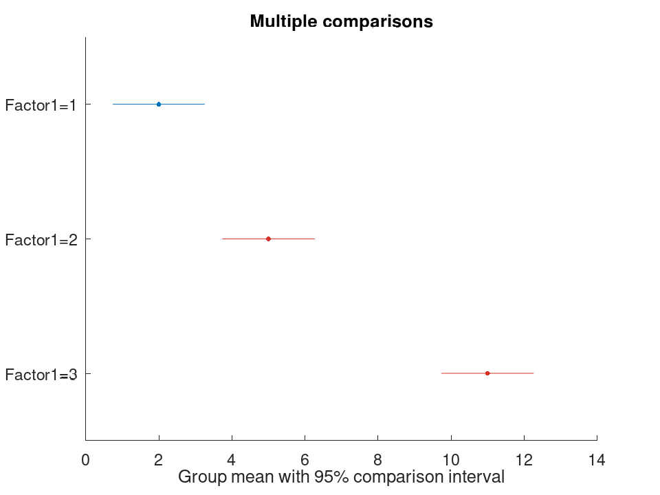
 plotComparisons (aov);

The anova class offers the following public methods:

anova: obj = anova (Y)
anova: obj = anova (factors, Y)
anova: obj = anova (tbl, Y)
anova: obj = anova (tbl, responseVarName)
anova: obj = anova (tbl, formula)
anova: obj = anova (…, name, value)

Y is a non-empty numeric response vector or matrix. factors contains grouping variables for vector responses and may be a grouping vector, a matrix of grouping variables, or a cell array of grouping vectors. If factors is omitted and Y is a matrix, columns of Y are treated as groups following anova1 matrix syntax.

tbl is a table whose variables contain factors. The response may be supplied separately, selected by variable name, or specified with a Wilkinson formula. 'FactorNames' can select a subset of table variables when a formula is not supplied.

Supported name-value arguments include 'ModelSpecification', 'SumOfSquaresType', 'FactorNames', 'CategoricalFactors', 'RandomFactors', 'ResponseName', 'Alpha', and 'Display'. Passing 'Reps' selects the balanced two-way anova2 backend when Y is a non-vector matrix.

Fit an ANOVA object and inspect component and summary statistics

 y = [1; 2; 3; 4; 5; 6; 10; 11; 12];
 g = [1; 1; 1; 2; 2; 2; 3; 3; 3];
 aov = anova (g, y, 'FactorNames', {'Treatment'});
 component = stats (aov)

component =
  3x5 table

                 SumOfSquares    DF    MeanSquares     F       pValue       
                 ____________    __    ___________    ___    ___________    

    Treatment             126     2             63     63    9.39144e-05    
    Error                   6     6              1    NaN            NaN    
    Total                 132     8            NaN    NaN            NaN

 summary_table = stats (aov, 'summary')

summary_table =
  4x5 table

                  SumOfSquares    DF    MeanSquares     F       pValue       
                  ____________    __    ___________    ___    ___________    

    Linear                 126     2             63     63    9.39144e-05    
    Regression             126     2             63     63    9.39144e-05    
    Error                    6     6              1    NaN            NaN    
    Total                  132     8           16.5    NaN            NaN

Estimate group means and perform post-hoc comparisons

 y = [1; 2; 3; 4; 5; 6; 10; 11; 12];
 g = [1; 1; 1; 2; 2; 2; 3; 3; 3];
 aov = anova (g, y, 'SumOfSquaresType', 'two');
 means = groupmeans (aov)

means =
  3x5 table

    Factor1    Mean      SE       MeanLower    MeanUpper    
    _______    ____    _______    _________    _________    

          1       2    0.57735     0.587275      3.41273    
          2       5    0.57735      3.58727      6.41273    
          3      11    0.57735      9.58727      12.4127

 comparisons = multcompare (aov, 'display', 'off')

comparisons =
  3x6 table

    Group1    Group2    MeanDifference    MeanDifferenceLower    MeanDifferenceUpper     pValue     
    ______    ______    ______________    ___________________    ___________________    ________    

         1         2                -3                -5.5039              -0.496098    0.024129    
         1         3                -9               -11.5039                -6.4961     8.3e-05    
         2         3                -6                -8.5039                -3.4961    0.000776

Plot multiple-comparison intervals

 y = [1; 2; 3; 4; 5; 6; 10; 11; 12];
 g = [1; 1; 1; 2; 2; 2; 3; 3; 3];
 aov = anova (g, y, 'SumOfSquaresType', 'two');
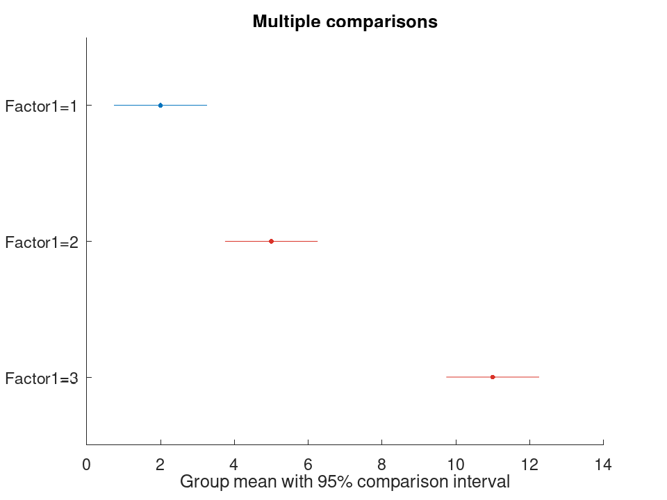
 plotComparisons (aov);

anova: s = stats (obj)
anova: s = stats (obj, type)
anova: s = stats (obj, "Component", sstype)
anova: [s, ems] = stats (…)

With no type, or with "component", return statistics for each model term, error, and total. With "summary", group terms into linear, nonlinear, and regression rows. Replicated continuous designs also report lack-of-fit and pure-error statistics.

The "Component" form computes the component table using sstype, which must be "one", "two", "three", or "hierarchical". This request does not change the object’s read-only SumOfSquaresType property. The second output ems contains expected mean-square information for each model term and the error term. Its variables are Type, ExpectedMeanSquares, MeanSquaresDenominator, DFDenominator, and FDenominator.

Fit an ANOVA object and inspect component and summary statistics

 y = [1; 2; 3; 4; 5; 6; 10; 11; 12];
 g = [1; 1; 1; 2; 2; 2; 3; 3; 3];
 aov = anova (g, y, 'FactorNames', {'Treatment'});
 component = stats (aov)

component =
  3x5 table

                 SumOfSquares    DF    MeanSquares     F       pValue       
                 ____________    __    ___________    ___    ___________    

    Treatment             126     2             63     63    9.39144e-05    
    Error                   6     6              1    NaN            NaN    
    Total                 132     8            NaN    NaN            NaN

 summary_table = stats (aov, 'summary')

summary_table =
  4x5 table

                  SumOfSquares    DF    MeanSquares     F       pValue       
                  ____________    __    ___________    ___    ___________    

    Linear                 126     2             63     63    9.39144e-05    
    Regression             126     2             63     63    9.39144e-05    
    Error                    6     6              1    NaN            NaN    
    Total                  132     8           16.5    NaN            NaN

Estimate group means and perform post-hoc comparisons

 y = [1; 2; 3; 4; 5; 6; 10; 11; 12];
 g = [1; 1; 1; 2; 2; 2; 3; 3; 3];
 aov = anova (g, y, 'SumOfSquaresType', 'two');
 means = groupmeans (aov)

means =
  3x5 table

    Factor1    Mean      SE       MeanLower    MeanUpper    
    _______    ____    _______    _________    _________    

          1       2    0.57735     0.587275      3.41273    
          2       5    0.57735      3.58727      6.41273    
          3      11    0.57735      9.58727      12.4127

 comparisons = multcompare (aov, 'display', 'off')

comparisons =
  3x6 table

    Group1    Group2    MeanDifference    MeanDifferenceLower    MeanDifferenceUpper     pValue     
    ______    ______    ______________    ___________________    ___________________    ________    

         1         2                -3               -5.50055              -0.499452    0.024222    
         1         3                -9               -11.5005               -6.49945     8.8e-05    
         2         3                -6               -8.50055               -3.49945    0.000767

Plot multiple-comparison intervals

 y = [1; 2; 3; 4; 5; 6; 10; 11; 12];
 g = [1; 1; 1; 2; 2; 2; 3; 3; 3];
 aov = anova (g, y, 'SumOfSquaresType', 'two');
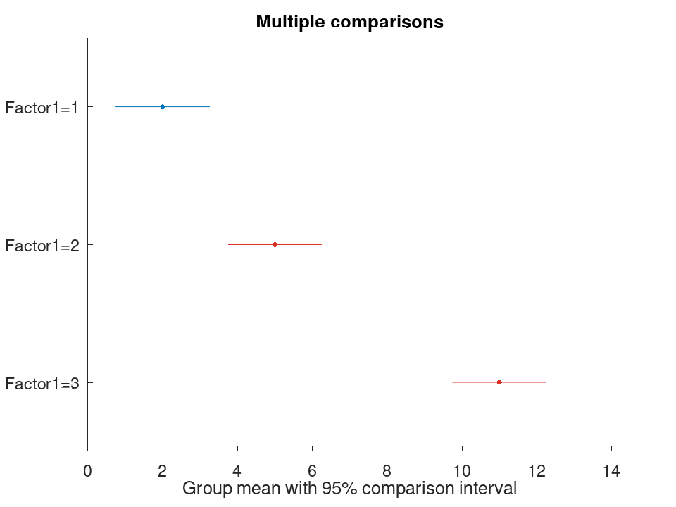
 plotComparisons (aov);

anova: means = groupmeans (obj)
anova: means = groupmeans (obj, factors)

The returned value is a table with one row per factor-level combination and columns for the level, mean, standard error, and confidence bounds.

Fit an ANOVA object and inspect component and summary statistics

 y = [1; 2; 3; 4; 5; 6; 10; 11; 12];
 g = [1; 1; 1; 2; 2; 2; 3; 3; 3];
 aov = anova (g, y, 'FactorNames', {'Treatment'});
 component = stats (aov)

component =
  3x5 table

                 SumOfSquares    DF    MeanSquares     F       pValue       
                 ____________    __    ___________    ___    ___________    

    Treatment             126     2             63     63    9.39144e-05    
    Error                   6     6              1    NaN            NaN    
    Total                 132     8            NaN    NaN            NaN

 summary_table = stats (aov, 'summary')

summary_table =
  4x5 table

                  SumOfSquares    DF    MeanSquares     F       pValue       
                  ____________    __    ___________    ___    ___________    

    Linear                 126     2             63     63    9.39144e-05    
    Regression             126     2             63     63    9.39144e-05    
    Error                    6     6              1    NaN            NaN    
    Total                  132     8           16.5    NaN            NaN

Estimate group means and perform post-hoc comparisons

 y = [1; 2; 3; 4; 5; 6; 10; 11; 12];
 g = [1; 1; 1; 2; 2; 2; 3; 3; 3];
 aov = anova (g, y, 'SumOfSquaresType', 'two');
 means = groupmeans (aov)

means =
  3x5 table

    Factor1    Mean      SE       MeanLower    MeanUpper    
    _______    ____    _______    _________    _________    

          1       2    0.57735     0.587275      3.41273    
          2       5    0.57735      3.58727      6.41273    
          3      11    0.57735      9.58727      12.4127

 comparisons = multcompare (aov, 'display', 'off')

comparisons =
  3x6 table

    Group1    Group2    MeanDifference    MeanDifferenceLower    MeanDifferenceUpper     pValue     
    ______    ______    ______________    ___________________    ___________________    ________    

         1         2                -3               -5.50203              -0.497971    0.024244    
         1         3                -9                -11.502               -6.49797     7.1e-05    
         2         3                -6               -8.50203               -3.49797    0.000726

Plot multiple-comparison intervals

 y = [1; 2; 3; 4; 5; 6; 10; 11; 12];
 g = [1; 1; 1; 2; 2; 2; 3; 3; 3];
 aov = anova (g, y, 'SumOfSquaresType', 'two');
 plotComparisons (aov);

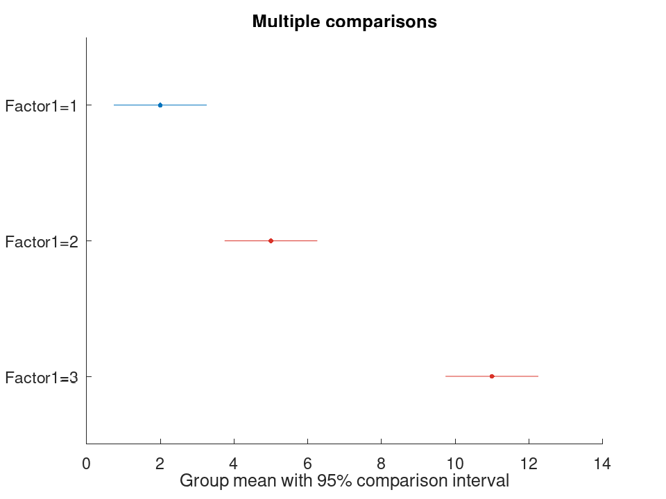
anova: boxchart (obj)
anova: h = boxchart (obj, …)

This method uses boxplot as the graphics backend in Octave and returns the native box graphics handles. A target axes may be supplied as the first optional argument.

Fit an ANOVA object and inspect component and summary statistics

 y = [1; 2; 3; 4; 5; 6; 10; 11; 12];
 g = [1; 1; 1; 2; 2; 2; 3; 3; 3];
 aov = anova (g, y, 'FactorNames', {'Treatment'});
 component = stats (aov)

component =
  3x5 table

                 SumOfSquares    DF    MeanSquares     F       pValue       
                 ____________    __    ___________    ___    ___________    

    Treatment             126     2             63     63    9.39144e-05    
    Error                   6     6              1    NaN            NaN    
    Total                 132     8            NaN    NaN            NaN

 summary_table = stats (aov, 'summary')

summary_table =
  4x5 table

                  SumOfSquares    DF    MeanSquares     F       pValue       
                  ____________    __    ___________    ___    ___________    

    Linear                 126     2             63     63    9.39144e-05    
    Regression             126     2             63     63    9.39144e-05    
    Error                    6     6              1    NaN            NaN    
    Total                  132     8           16.5    NaN            NaN

Estimate group means and perform post-hoc comparisons

 y = [1; 2; 3; 4; 5; 6; 10; 11; 12];
 g = [1; 1; 1; 2; 2; 2; 3; 3; 3];
 aov = anova (g, y, 'SumOfSquaresType', 'two');
 means = groupmeans (aov)

means =
  3x5 table

    Factor1    Mean      SE       MeanLower    MeanUpper    
    _______    ____    _______    _________    _________    

          1       2    0.57735     0.587275      3.41273    
          2       5    0.57735      3.58727      6.41273    
          3      11    0.57735      9.58727      12.4127

 comparisons = multcompare (aov, 'display', 'off')

comparisons =
  3x6 table

    Group1    Group2    MeanDifference    MeanDifferenceLower    MeanDifferenceUpper     pValue     
    ______    ______    ______________    ___________________    ___________________    ________    

         1         2                -3               -5.50645              -0.493546    0.024266    
         1         3                -9               -11.5065               -6.49355     9.2e-05    
         2         3                -6               -8.50645               -3.49355    0.000793

Plot multiple-comparison intervals

 y = [1; 2; 3; 4; 5; 6; 10; 11; 12];
 g = [1; 1; 1; 2; 2; 2; 3; 3; 3];
 aov = anova (g, y, 'SumOfSquaresType', 'two');
 plotComparisons (aov);

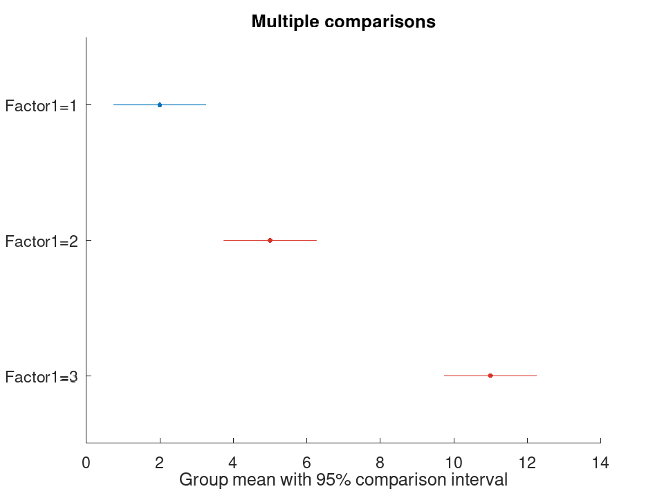
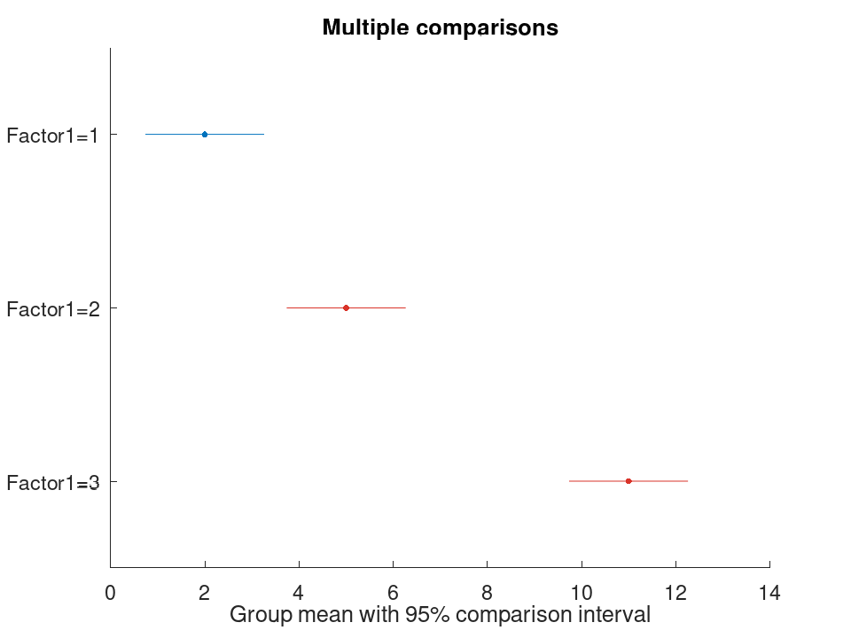
anova: plotComparisons (obj)
anova: h = plotComparisons (obj, …)

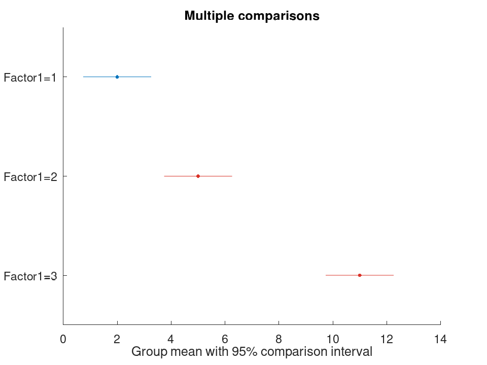
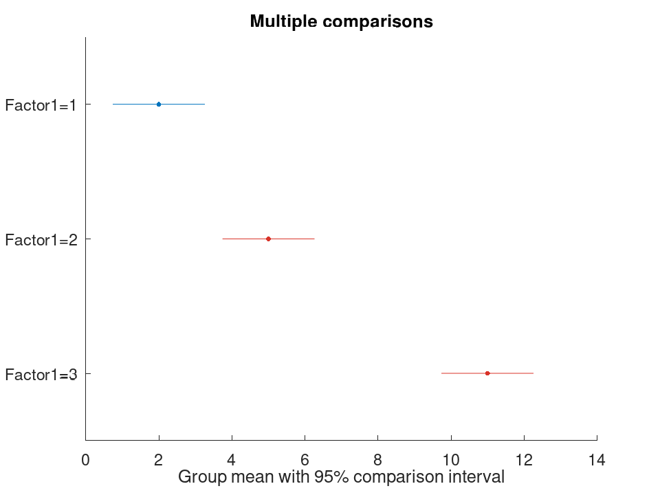
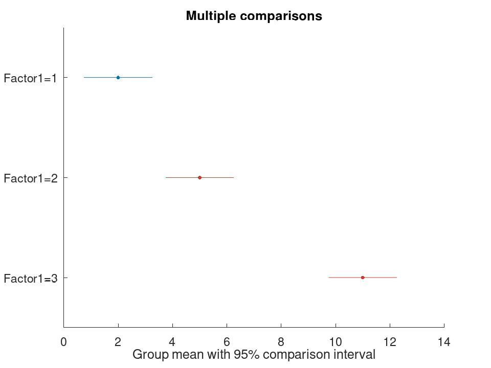
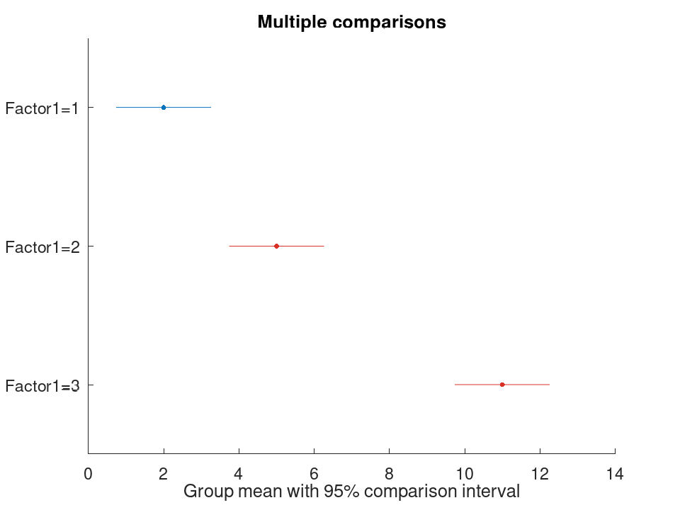
Clicking a group highlights it and distinguishes groups whose adjusted comparison is significant at the requested alpha level. A target axes may be supplied as the first optional argument.

Fit an ANOVA object and inspect component and summary statistics

 y = [1; 2; 3; 4; 5; 6; 10; 11; 12];
 g = [1; 1; 1; 2; 2; 2; 3; 3; 3];
 aov = anova (g, y, 'FactorNames', {'Treatment'});
 component = stats (aov)

component =
  3x5 table

                 SumOfSquares    DF    MeanSquares     F       pValue       
                 ____________    __    ___________    ___    ___________    

    Treatment             126     2             63     63    9.39144e-05    
    Error                   6     6              1    NaN            NaN    
    Total                 132     8            NaN    NaN            NaN

 summary_table = stats (aov, 'summary')

summary_table =
  4x5 table

                  SumOfSquares    DF    MeanSquares     F       pValue       
                  ____________    __    ___________    ___    ___________    

    Linear                 126     2             63     63    9.39144e-05    
    Regression             126     2             63     63    9.39144e-05    
    Error                    6     6              1    NaN            NaN    
    Total                  132     8           16.5    NaN            NaN

Estimate group means and perform post-hoc comparisons

 y = [1; 2; 3; 4; 5; 6; 10; 11; 12];
 g = [1; 1; 1; 2; 2; 2; 3; 3; 3];
 aov = anova (g, y, 'SumOfSquaresType', 'two');
 means = groupmeans (aov)

means =
  3x5 table

    Factor1    Mean      SE       MeanLower    MeanUpper    
    _______    ____    _______    _________    _________    

          1       2    0.57735     0.587275      3.41273    
          2       5    0.57735      3.58727      6.41273    
          3      11    0.57735      9.58727      12.4127

 comparisons = multcompare (aov, 'display', 'off')

comparisons =
  3x6 table

    Group1    Group2    MeanDifference    MeanDifferenceLower    MeanDifferenceUpper     pValue     
    ______    ______    ______________    ___________________    ___________________    ________    

         1         2                -3               -5.50636              -0.493644    0.024285    
         1         3                -9               -11.5064               -6.49364     7.6e-05    
         2         3                -6               -8.50636               -3.49364    0.000781

Plot multiple-comparison intervals

 y = [1; 2; 3; 4; 5; 6; 10; 11; 12];
 g = [1; 1; 1; 2; 2; 2; 3; 3; 3];
 aov = anova (g, y, 'SumOfSquaresType', 'two');
 plotComparisons (aov);

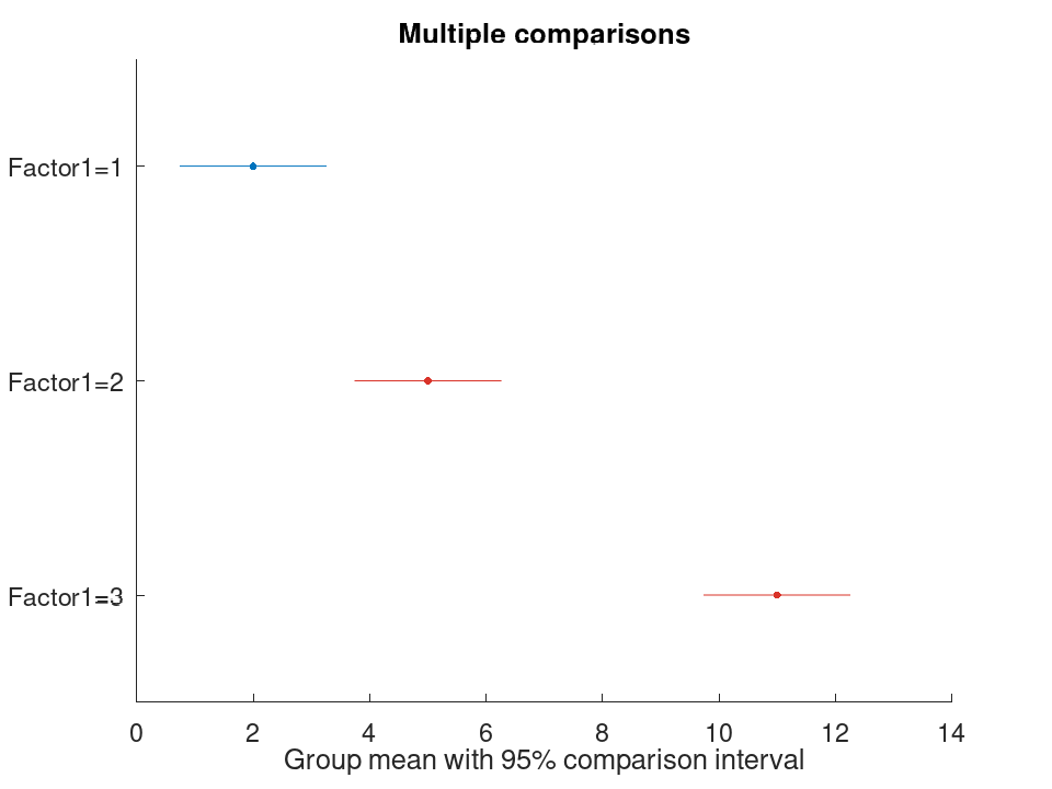
anova: v = varianceComponent (obj)
anova: v = varianceComponent (obj, …)

Fit an ANOVA object and inspect component and summary statistics

 y = [1; 2; 3; 4; 5; 6; 10; 11; 12];
 g = [1; 1; 1; 2; 2; 2; 3; 3; 3];
 aov = anova (g, y, 'FactorNames', {'Treatment'});
 component = stats (aov)

component =
  3x5 table

                 SumOfSquares    DF    MeanSquares     F       pValue       
                 ____________    __    ___________    ___    ___________    

    Treatment             126     2             63     63    9.39144e-05    
    Error                   6     6              1    NaN            NaN    
    Total                 132     8            NaN    NaN            NaN

 summary_table = stats (aov, 'summary')

summary_table =
  4x5 table

                  SumOfSquares    DF    MeanSquares     F       pValue       
                  ____________    __    ___________    ___    ___________    

    Linear                 126     2             63     63    9.39144e-05    
    Regression             126     2             63     63    9.39144e-05    
    Error                    6     6              1    NaN            NaN    
    Total                  132     8           16.5    NaN            NaN

Estimate group means and perform post-hoc comparisons

 y = [1; 2; 3; 4; 5; 6; 10; 11; 12];
 g = [1; 1; 1; 2; 2; 2; 3; 3; 3];
 aov = anova (g, y, 'SumOfSquaresType', 'two');
 means = groupmeans (aov)

means =
  3x5 table

    Factor1    Mean      SE       MeanLower    MeanUpper    
    _______    ____    _______    _________    _________    

          1       2    0.57735     0.587275      3.41273    
          2       5    0.57735      3.58727      6.41273    
          3      11    0.57735      9.58727      12.4127

 comparisons = multcompare (aov, 'display', 'off')

comparisons =
  3x6 table

    Group1    Group2    MeanDifference    MeanDifferenceLower    MeanDifferenceUpper     pValue     
    ______    ______    ______________    ___________________    ___________________    ________    

         1         2                -3               -5.51279              -0.487212    0.024487    
         1         3                -9               -11.5128               -6.48721    0.000103    
         2         3                -6               -8.51279               -3.48721    0.000851

Plot multiple-comparison intervals

 y = [1; 2; 3; 4; 5; 6; 10; 11; 12];
 g = [1; 1; 1; 2; 2; 2; 3; 3; 3];
 aov = anova (g, y, 'SumOfSquaresType', 'two');
 plotComparisons (aov);

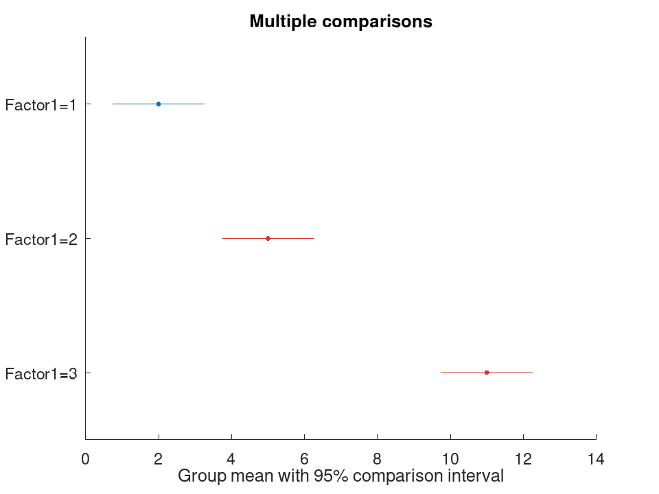
anova: m = multcompare (obj)
anova: m = multcompare (obj, factors)
anova: m = multcompare (…, name, value)

The returned table contains the compared groups, estimated mean difference, confidence limits, and p-value. The default critical value type is "tukey-kramer".

Fit an ANOVA object and inspect component and summary statistics

 y = [1; 2; 3; 4; 5; 6; 10; 11; 12];
 g = [1; 1; 1; 2; 2; 2; 3; 3; 3];
 aov = anova (g, y, 'FactorNames', {'Treatment'});
 component = stats (aov)

component =
  3x5 table

                 SumOfSquares    DF    MeanSquares     F       pValue       
                 ____________    __    ___________    ___    ___________    

    Treatment             126     2             63     63    9.39144e-05    
    Error                   6     6              1    NaN            NaN    
    Total                 132     8            NaN    NaN            NaN

 summary_table = stats (aov, 'summary')

summary_table =
  4x5 table

                  SumOfSquares    DF    MeanSquares     F       pValue       
                  ____________    __    ___________    ___    ___________    

    Linear                 126     2             63     63    9.39144e-05    
    Regression             126     2             63     63    9.39144e-05    
    Error                    6     6              1    NaN            NaN    
    Total                  132     8           16.5    NaN            NaN

Estimate group means and perform post-hoc comparisons

 y = [1; 2; 3; 4; 5; 6; 10; 11; 12];
 g = [1; 1; 1; 2; 2; 2; 3; 3; 3];
 aov = anova (g, y, 'SumOfSquaresType', 'two');
 means = groupmeans (aov)

means =
  3x5 table

    Factor1    Mean      SE       MeanLower    MeanUpper    
    _______    ____    _______    _________    _________    

          1       2    0.57735     0.587275      3.41273    
          2       5    0.57735      3.58727      6.41273    
          3      11    0.57735      9.58727      12.4127

 comparisons = multcompare (aov, 'display', 'off')

comparisons =
  3x6 table

    Group1    Group2    MeanDifference    MeanDifferenceLower    MeanDifferenceUpper     pValue     
    ______    ______    ______________    ___________________    ___________________    ________    

         1         2                -3               -5.50723              -0.492774    0.024243    
         1         3                -9               -11.5072               -6.49277     9.1e-05    
         2         3                -6               -8.50723               -3.49277    0.000773

Plot multiple-comparison intervals

 y = [1; 2; 3; 4; 5; 6; 10; 11; 12];
 g = [1; 1; 1; 2; 2; 2; 3; 3; 3];
 aov = anova (g, y, 'SumOfSquaresType', 'two');
 plotComparisons (aov);

Examples

 y = [1; 2; 3; 4; 5; 6; 10; 11; 12];
 g = [1; 1; 1; 2; 2; 2; 3; 3; 3];
 aov = anova (g, y, 'FactorNames', {'Treatment'});
 component = stats (aov)

component =
  3x5 table

                 SumOfSquares    DF    MeanSquares     F       pValue       
                 ____________    __    ___________    ___    ___________    

    Treatment             126     2             63     63    9.39144e-05    
    Error                   6     6              1    NaN            NaN    
    Total                 132     8            NaN    NaN            NaN

 summary_table = stats (aov, 'summary')

summary_table =
  4x5 table

                  SumOfSquares    DF    MeanSquares     F       pValue       
                  ____________    __    ___________    ___    ___________    

    Linear                 126     2             63     63    9.39144e-05    
    Regression             126     2             63     63    9.39144e-05    
    Error                    6     6              1    NaN            NaN    
    Total                  132     8           16.5    NaN            NaN

 y = [1; 2; 3; 4; 5; 6; 10; 11; 12];
 g = [1; 1; 1; 2; 2; 2; 3; 3; 3];
 aov = anova (g, y, 'SumOfSquaresType', 'two');
 means = groupmeans (aov)

means =
  3x5 table

    Factor1    Mean      SE       MeanLower    MeanUpper    
    _______    ____    _______    _________    _________    

          1       2    0.57735     0.587275      3.41273    
          2       5    0.57735      3.58727      6.41273    
          3      11    0.57735      9.58727      12.4127

 comparisons = multcompare (aov, 'display', 'off')

comparisons =
  3x6 table

    Group1    Group2    MeanDifference    MeanDifferenceLower    MeanDifferenceUpper     pValue     
    ______    ______    ______________    ___________________    ___________________    ________    

         1         2                -3               -5.50064               -0.49936    0.024081    
         1         3                -9               -11.5006               -6.49936     8.2e-05    
         2         3                -6               -8.50064               -3.49936     0.00086

 y = [1; 2; 3; 4; 5; 6; 10; 11; 12];
 g = [1; 1; 1; 2; 2; 2; 3; 3; 3];
 aov = anova (g, y, 'SumOfSquaresType', 'two');
 plotComparisons (aov);

Categories &

Functions List

Descriptive Statistics

Descriptive Statistics

Data Manipulation

Data Manipulation

Hypothesis Testing

Hypothesis Testing

Experimental Design

Experimental Design

Regression

Regression

Supervised Learning

Supervised Learning

Clustering

Clustering

Nearest Neighbors

Nearest Neighbors

Anomaly Detection

Anomaly Detection

Dimensionality Reduction

Dimensionality Reduction

Model Evaluation

Model Evaluation

Markov Models

Markov Models

Random Sampling

Random Sampling

Distribution Classes

Distribution Classes

Distribution Fitting

Distribution Fitting

Distribution Functions

Distribution Functions

Distribution Statistics

Distribution Statistics

Distribution Wrappers

Distribution Wrappers

Plotting

Plotting

I/O

I/O

Utilities

Utilities

Class Definition: anova

statistics: anova

Y

Factors

Formula

FactorNames

ExpandedFactorNames

SumOfSquaresType

RandomFactors

CategoricalFactors

ResponseName

NumObservations

Coefficients

Residuals

Metrics

anova

anova: obj = anova (Y)

anova: obj = anova (factors, Y)

anova: obj = anova (tbl, Y)

anova: obj = anova (tbl, responseVarName)

anova: obj = anova (tbl, formula)

anova: obj = anova (…, name, value)

stats

anova: s = stats (obj)

anova: s = stats (obj, type)

anova: s = stats (obj, "Component", sstype)

anova: [s, ems] = stats (…)

groupmeans

anova: means = groupmeans (obj)

anova: means = groupmeans (obj, factors)

boxchart

anova: boxchart (obj)

anova: h = boxchart (obj, …)

plotComparisons

anova: plotComparisons (obj)

anova: h = plotComparisons (obj, …)

Class Definition: `anova`

`Y`

`Factors`

`Formula`

`FactorNames`

`ExpandedFactorNames`

`SumOfSquaresType`

`RandomFactors`

`CategoricalFactors`

`ResponseName`

`NumObservations`

`Coefficients`

`Residuals`

`Metrics`

`anova`

`anova: obj = anova (Y)`

`anova: obj = anova (factors, Y)`

`anova: obj = anova (tbl, Y)`

`anova: obj = anova (tbl, responseVarName)`

`anova: obj = anova (tbl, formula)`

`anova: obj = anova (…, name, value)`

`stats`

`anova: s = stats (obj)`

`anova: s = stats (obj, type)`

`anova: s = stats (obj, "Component", sstype)`

`anova: [s, ems] = stats (…)`

`groupmeans`

`anova: means = groupmeans (obj)`

`anova: means = groupmeans (obj, factors)`

`boxchart`

`anova: boxchart (obj)`

`anova: h = boxchart (obj, …)`

`plotComparisons`

`anova: plotComparisons (obj)`

`anova: h = plotComparisons (obj, …)`

`varianceComponent`

`anova: v = varianceComponent (obj)`

`anova: v = varianceComponent (obj, …)`

`multcompare`

`anova: m = multcompare (obj)`

`anova: m = multcompare (obj, factors)`

`anova: m = multcompare (…, name, value)`