Categories &
Functions List
- adtest
- anova
- anova1
- anova2
- anovan
- ansaribradley
- barttest
- binotest
- chi2gof
- chi2test
- correlation_test
- detectdrift
- dwtest
- fishertest
- friedman
- hotelling_t2test
- hotelling_t2test2
- jbtest
- knntest
- kruskalwallis
- kstest
- kstest2
- lillietest
- manova1
- mcnemar_test
- meanEffectSize
- mmdtest
- multcompare
- ranksum
- regression_ftest
- regression_ttest
- runstest
- signrank
- signtest
- stats.drift.DriftDiagnostics
- swtest
- ttest
- ttest2
- vartest
- vartest2
- vartestn
- ztest
- ztest2
- CompactLinearModel
- CoxModel
- coxphfit
- fitcox
- fitglm
- fitglme
- fitlm
- fitlme
- fitlmematrix
- fitnlm
- fitrm
- GeneralizedLinearMixedModel
- GeneralizedLinearModel
- glmfit
- glmval
- invpred
- lasso
- lassoglm
- LinearFormula
- LinearMixedModel
- LinearModel
- logistic_regression
- mnrfit
- mnrval
- monotone_smooth
- mvregress
- mvregresslike
- nlinfit
- nlparci
- nlpredci
- NonLinearModel
- plsregress
- regress
- regress_gp
- RepeatedMeasuresModel
- ridge
- robustfit
- stepwisefit
- stepwiseglm
- stepwiselm
- ClassificationBaggedEnsemble
- ClassificationDiscriminant
- ClassificationECOC
- ClassificationEnsemble
- ClassificationGAM
- ClassificationKernel
- ClassificationKNN
- ClassificationLinear
- ClassificationNaiveBayes
- ClassificationNeuralNetwork
- ClassificationPartitionedECOC
- ClassificationPartitionedEnsemble
- ClassificationPartitionedKernel
- ClassificationPartitionedLinear
- ClassificationPartitionedModel
- ClassificationSVM
- ClassificationTree
- CompactClassificationDiscriminant
- CompactClassificationECOC
- CompactClassificationEnsemble
- CompactClassificationGAM
- CompactClassificationNaiveBayes
- CompactClassificationNeuralNetwork
- CompactClassificationSVM
- CompactClassificationTree
- CompactRegressionGAM
- CompactRegressionEnsemble
- CompactRegressionGP
- CompactRegressionNeuralNetwork
- CompactRegressionSVM
- CompactRegressionTree
- CompactTreeBagger
- designecoc
- fcnnpredict
- fcnntrain
- fitcdiscr
- fitcecoc
- fitcensemble
- fitcgam
- fitckernel
- fitcknn
- fitclinear
- fitcnb
- fitcnet
- fitcsvm
- fitctree
- fitrensemble
- fitrgam
- fitrgp
- fitrkernel
- fitrlinear
- fitrnet
- fitrsvm
- fitrtree
- gamboostinter
- gamboostpairs
- gamboostpredict
- gamboosttrain
- gampredict
- gamtrain
- partialDependence
- plotPartialDependence
- PredictiveModel
- RegressionBaggedEnsemble
- RegressionEnsemble
- RegressionGAM
- RegressionGP
- RegressionKernel
- RegressionLinear
- RegressionNeuralNetwork
- RegressionPartitionedEnsemble
- RegressionPartitionedKernel
- RegressionPartitionedLinear
- RegressionPartitionedModel
- RegressionSVM
- RegressionTree
- lime
- shapley
- svmpredict
- svmtrain
- templateDiscriminant
- templateEnsemble
- templateKernel
- templateKNN
- templateLinear
- templateNaiveBayes
- templateSVM
- templateTree
- TreeBagger
- treepredict
- treetrain
- paretotails
- prob.ProbabilityDistribution
- prob.BetaDistribution
- prob.BinomialDistribution
- prob.BirnbaumSaundersDistribution
- prob.BurrDistribution
- prob.ExponentialDistribution
- prob.ExtremeValueDistribution
- prob.GammaDistribution
- prob.GeneralizedExtremeValueDistribution
- prob.GeneralizedParetoDistribution
- prob.HalfNormalDistribution
- prob.InverseGaussianDistribution
- prob.KernelDistribution
- prob.LogisticDistribution
- prob.LoglogisticDistribution
- prob.LognormalDistribution
- prob.LoguniformDistribution
- prob.MultinomialDistribution
- prob.NakagamiDistribution
- prob.NegativeBinomialDistribution
- prob.NormalDistribution
- prob.PiecewiseLinearDistribution
- prob.PoissonDistribution
- prob.RayleighDistribution
- prob.RicianDistribution
- prob.StableDistribution
- prob.tLocationScaleDistribution
- prob.TriangularDistribution
- prob.UniformDistribution
- prob.WeibullDistribution
- betafit
- betalike
- binofit
- binolike
- bisafit
- bisalike
- burrfit
- burrlike
- copulafit
- evfit
- evlike
- expfit
- explike
- gamfit
- gamlike
- geofit
- gevfit
- gevlike
- gevfit_lmom
- gpfit
- gplike
- gumbelfit
- gumbellike
- hnfit
- hnlike
- invgfit
- invglike
- logifit
- logilike
- loglfit
- logllike
- lognfit
- lognlike
- nakafit
- nakalike
- nbinfit
- nbinlike
- normfit
- normlike
- poissfit
- poisslike
- raylfit
- rayllike
- ricefit
- ricelike
- stblfit
- stbllike
- tlsfit
- tlslike
- unidfit
- unifit
- wblfit
- wbllike
- betacdf
- betainv
- betapdf
- betarnd
- binocdf
- binoinv
- binopdf
- binornd
- bisacdf
- bisainv
- bisapdf
- bisarnd
- burrcdf
- burrinv
- burrpdf
- burrrnd
- bvncdf
- bvtcdf
- cauchycdf
- cauchyinv
- cauchypdf
- cauchyrnd
- chi2cdf
- chi2inv
- chi2pdf
- chi2rnd
- copulacdf
- copulapdf
- copularnd
- evcdf
- evinv
- evpdf
- evrnd
- expcdf
- expinv
- exppdf
- exprnd
- fcdf
- finv
- fpdf
- frnd
- gamcdf
- gaminv
- gampdf
- gamrnd
- geocdf
- geoinv
- geopdf
- geornd
- gevcdf
- gevinv
- gevpdf
- gevrnd
- gpcdf
- gpinv
- gppdf
- gprnd
- gumbelcdf
- gumbelinv
- gumbelpdf
- gumbelrnd
- hncdf
- hninv
- hnpdf
- hnrnd
- hygecdf
- hygeinv
- hygepdf
- hygernd
- invgcdf
- invginv
- invgpdf
- invgrnd
- iwishpdf
- iwishrnd
- jsucdf
- jsupdf
- laplacecdf
- laplaceinv
- laplacepdf
- laplacernd
- logicdf
- logiinv
- logipdf
- logirnd
- loglcdf
- loglinv
- loglpdf
- loglrnd
- logncdf
- logninv
- lognpdf
- lognrnd
- mnpdf
- mnrnd
- mvncdf
- mvnpdf
- mvnrnd
- mvtcdf
- mvtpdf
- mvtrnd
- nakacdf
- nakainv
- nakapdf
- nakarnd
- nbincdf
- nbininv
- nbinpdf
- nbinrnd
- ncfcdf
- ncfinv
- ncfpdf
- ncfrnd
- nctcdf
- nctinv
- nctpdf
- nctrnd
- ncx2cdf
- ncx2inv
- ncx2pdf
- ncx2rnd
- normcdf
- norminv
- normpdf
- normrnd
- plcdf
- plinv
- plpdf
- plrnd
- poisscdf
- poissinv
- poisspdf
- poissrnd
- raylcdf
- raylinv
- raylpdf
- raylrnd
- ricecdf
- riceinv
- ricepdf
- ricernd
- stblcdf
- stblinv
- stblpdf
- stblrnd
- stdrcdf
- stdrinv
- stdrpdf
- stdrrnd
- tcdf
- tinv
- tpdf
- trnd
- tlscdf
- tlsinv
- tlspdf
- tlsrnd
- tricdf
- triinv
- tripdf
- trirnd
- unidcdf
- unidinv
- unidpdf
- unidrnd
- unifcdf
- unifinv
- unifpdf
- unifrnd
- vmcdf
- vminv
- vmpdf
- vmrnd
- wblcdf
- wblinv
- wblpdf
- wblrnd
- wienrnd
- wishpdf
- wishrnd
- betastat
- binostat
- bisastat
- burrstat
- chi2stat
- copulaparam
- copulastat
- evstat
- expstat
- fstat
- gamstat
- geostat
- gevstat
- gpstat
- gumbelstat
- hnstat
- hygestat
- invgstat
- logistat
- loglstat
- lognstat
- nakastat
- nbinstat
- ncfstat
- nctstat
- ncx2stat
- normstat
- plstat
- poisstat
- raylstat
- ricestat
- stdrstat
- tlsstat
- tristat
- tstat
- unidstat
- unifstat
- wblstat
- andrewsplot
- bar3
- bar3h
- biplot
- boxchart
- boxplot
- cdfplot
- dendrogram
- ecdfhist
- einstein
- gardnerAltmanPlot
- glyphplot
- gplotmatrix
- gscatter
- heatmap
- hist3
- histfit
- manovacluster
- normplot
- parallelcoords
- parallelplot
- ppplot
- probplot
- qqplot
- scatterhist
- scatterhistogram
- silhouette
- stats.chart.BoxChart
- stats.chart.HeatmapChart
- stats.chart.ParallelCoordinatesPlot
- stats.chart.ScatterHistogramChart
- swarmchart
- violin
- wblplot
Function Reference: fitrsvm
statistics: Mdl = fitrsvm (X, Y)
statistics: Mdl = fitrsvm (Tbl, ResponseVarName)
statistics: Mdl = fitrsvm (Tbl, formula)
statistics: Mdl = fitrsvm (Tbl, Y)
statistics: Mdl = fitrsvm (…, name, value)
Fit a support vector machine regression model.
Mdl = fitrsvm (X, Y) returns a support vector
regression model, Mdl, with X being the predictor data and
Y the continuous response of the observations in X.
- X must be an NxP numeric matrix of predictor data, where rows correspond to observations and columns to features or variables.
- Y must be an Nx1 numeric vector holding the response of the corresponding predictor data in X. Y must have the same number of rows as X.
The model is fitted by epsilon-insensitive regression: an error
smaller than Epsilon costs nothing, so only the observations
outside that tube become support vectors. Use fitcsvm where the
response names a class rather than a quantity.
Mdl = fitrsvm (…, name, value) returns a
model with additional options specified by Name-Value pair
arguments listed below.
Model Parameters
| Name | Value |
|---|---|
'Standardize' | A logical scalar indicating whether the
data in X should be centred and scaled before training. The same
transformation is applied by predict. The default is false. |
'CategoricalPredictors' | The predictors whose values are
levels, as indices, as a logical vector with one element per predictor, or as
'all'. Each is dummy coded in its place, one column of zeros and
ones per level seen in training, named as in 'x1 == 2' in
ExpandedPredictorNames, and the coded columns are not standardized.
An observation holding a level the training data did not has no prediction.
A predictor may be named rather than indexed, as a character matrix of one
padded name per row, a string array or a cellstr; a name must match an entry
of 'PredictorNames' exactly, its case included. |
'PredictorNames' | A cell array of character vectors specifying the predictor variable names, in the order they appear in X. |
'ResponseName' | A character vector specifying the name of
the response variable. The default is 'Y'. |
'ResponseTransform' | A character vector naming one of
'none', 'identity', 'exp' or 'log', or a
function handle of one argument, applied to the predicted response. The
default is 'none'. |
'Epsilon' | A non-negative scalar, the half-width of the
insensitive tube. The default is iqr (Y) / 13.49, a robust
estimate of a tenth of the response’s standard deviation, which is what
MATLAB uses; where that is zero it falls back to 0.1. |
'BoxConstraint' | A positive scalar bounding the dual
coefficients, the cost of an error outside the tube. The default is
iqr (Y) / 1.349 for a Gaussian kernel, or 1 where that is
zero, and 1 for any other kernel. |
'Weights' | A nonnegative single or double vector of
observation weights, one per row of X. An observation’s box
constraint is n times BoxConstraint times its weight, the
weights scaled to sum to one; standardization uses weighted means and
standard deviations, and a row of zero or missing weight is left out. The
model’s W keeps the class of the weights, while every computation
runs in double. The default is uniform. |
'KernelFunction' | A character vector naming the kernel,
one of 'linear', the default, 'rbf', 'gaussian',
'polynomial' or 'sigmoid'. |
'PolynomialOrder' | A positive integer, the order of the polynomial kernel. The default is 3. It is ignored by every other kernel. |
'KernelScale' | A positive scalar dividing every predictor
before any kernel is applied, as MATLAB does, so that with u and
v the divided predictors the kernels are u'v,
exp (-||u - v||^2), (1 + u'v)^q and tanh (u'v + c),
c being 'KernelOffset'. The default is 1. |
'KernelOffset' | A non-negative scalar, the constant c of the sigmoid kernel, which MATLAB does not have. MATLAB adds it to every element of the Gram matrix, which leaves the fitted model unchanged, so it changes no other kernel here. The default is 0. |
'SVMtype' | A character vector selecting the formulation,
either 'eps_svr', the default, or 'nu_svr'. MATLAB fits
only the epsilon form; 'nu_svr' is an Octave extension. |
'Nu' | A scalar in (0, 1] used by
'nu_svr', bounding the fraction of support vectors. The default
is 0.5. |
'CacheSize' | A positive scalar, the kernel cache in megabytes. The default is 1000. |
'Tolerance' | A non-negative scalar, the tolerance of the termination criterion. The default is 1e-6. |
'Shrinking' | Either 0 or 1, whether to use the shrinking heuristic. The default is 1. |
See also: RegressionSVM, fitcsvm, fitrnet, svmtrain, svmpredict
Source Code: fitrsvm
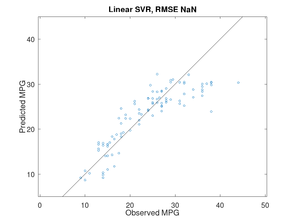
- Predict fuel economy from engine power and weight
 load carsmall
 X = [Horsepower, Weight];
 Mdl = fitrsvm (X, MPG, 'Standardize', true);
Rows carrying a missing value were dropped, so ask about the ones used
 used = Mdl.RowsUsed;
 yFit = predict (Mdl, X(used,:));
 plot (MPG(used), yFit, 'o', [5, 45], [5, 45], 'k-');
 axis equal;
 xlabel ('Observed MPG');
 ylabel ('Predicted MPG');
 title (sprintf ('Linear SVR, RMSE %.2f', sqrt (resubLoss (Mdl))));
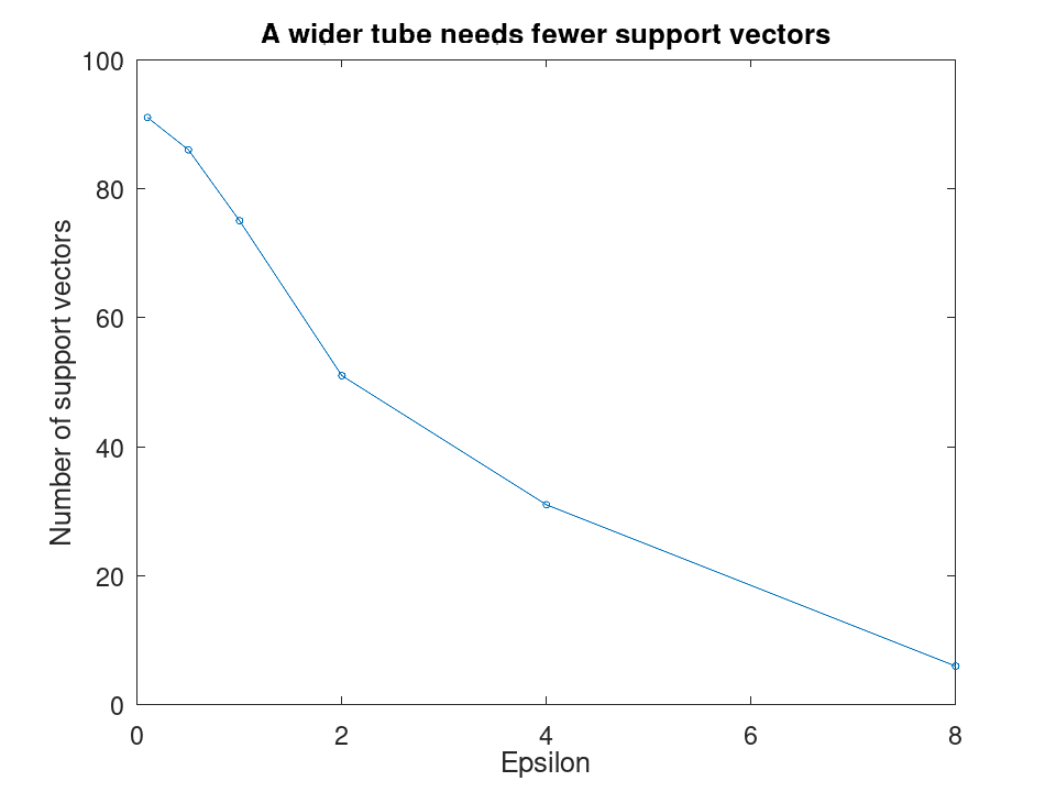
- The insensitive tube decides who becomes a support vector
Errors smaller than Epsilon cost nothing, so a wider tube is fitted by fewer observations and a narrower one by almost all of them.
 load carsmall
 X = [Horsepower, Weight];
 eps_ = [0.1, 0.5, 1, 2, 4, 8];
 nsv = zeros (size (eps_));
 for k = 1:numel (eps_)
   m = fitrsvm (X, MPG, 'Standardize', true, 'Epsilon', eps_(k));
   nsv(k) = sum (m.IsSupportVector);
 endfor
 plot (eps_, nsv, 'o-', 'linewidth', 1.5);
 xlabel ('Epsilon');
 ylabel ('Number of support vectors');
 title ('A wider tube needs fewer support vectors');
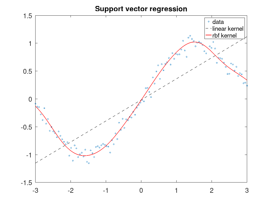
- A radial kernel fits a curve a linear one cannot
 rng (42);
 x = linspace (-3, 3, 120)';
 y = sin (x) + randn (120, 1) * 0.1;
 lin = fitrsvm (x, y);
 rbf = fitrsvm (x, y, 'KernelFunction', 'rbf', 'BoxConstraint', 10);
 plot (x, y, 'o', 'markersize', 4);
 hold on;
 plot (x, predict (lin, x), 'k--', 'linewidth', 1.5);
 plot (x, predict (rbf, x), 'r-', 'linewidth', 2);
 hold off;
 legend ({'data', 'linear kernel', 'rbf kernel'});
 title ('Support vector regression');
- With a linear kernel the model is a plain linear function
 load carsmall
 X = [Horsepower, Weight];
 Mdl = fitrsvm (X, MPG, 'Standardize', true);
 used = Mdl.RowsUsed;
 Xs = (X(used,:) - Mdl.Mu) ./ Mdl.Sigma;
 printf ('max |X*Beta + Bias - predict| = %g\n', ...
         max (abs (Xs * Mdl.Beta + Mdl.Bias - resubPredict (Mdl))));
max |X*Beta + Bias - predict| = 3.19744e-14
Fit from a table, and predict on one
 load fisheriris
 T = table (meas(:,2), meas(:,3), meas(:,4), meas(:,1), ...
            'VariableNames', {'SW', 'PL', 'PW', 'SL'});
 T.Wide = categorical (meas(:,2) > 3, [false true], {'narrow', 'wide'});
A model formula names the response and the predictors together, and holds main effects only
 Mdl = fitrsvm (T, 'SL ~ PL + Wide');
 Mdl.PredictorNames
ans =
  1x2 cell array

    {'PL'}    {'Wide'}
Mdl.ResponseName
ans = SL
Mdl.CategoricalPredictors
ans = 2
predict matches the table's variables by name, so a column the model was not fitted on is passed over
 yFit = predict (Mdl, T(1:5,:));
 yFit'
ans =

   4.9668   4.5483   4.9208   5.0127   4.9668