Statistics: CoxModel

Class Definition: `CoxModel`

statistics: CoxModel

Cox proportional hazards regression model class.

A CoxModel object encapsulates a Cox proportional hazards model of a survival time on one or more predictors, fitted by maximizing the Cox partial likelihood. It is the object counterpart of coxphfit and is normally created with the fitcox function.

The model states that an observation with predictor values x has hazard

$$ h(x, t) = h_0(t)\exp\left(\sum_{j=1}^{p} x_{j} b_j\right) $$

where $h_0(t)$ is an unspecified baseline hazard. The model carries no constant term: any constant is absorbed into that baseline.

The most useful properties are Coefficients (a table of estimates, standard errors, $z$ -statistics and p-values), Hazard (the estimated baseline cumulative hazard), LogLikelihood, Residuals, and the three p-values LikelihoodRatioTestPValue, ProportionalHazardsPValue and ProportionalHazardsPValueGlobal. Fitted models support the survival, hazardratio, coefci, linhyptest, plotSurvival and discardResiduals methods.

A categorical predictor expands to indicator columns, one per level bar the first, which the baseline hazard carries; the indicator columns are named name_level and enter the default baseline as zero, while a numeric predictor enters it as its mean.

ProportionalHazardsPValue is a Grambsch-Therneau test of each coefficient against the mid-ranks of the event times, and ProportionalHazardsPValueGlobal the same test taken over the whole model. A small p-value is evidence that the hazard ratio moves with time, which is what proportionality denies.

Deviations from MATLAB, all in naming. MATLAB derives the names reported by a fitted model from three different places and they need not agree with one another: with default predictor names its Formula reads 'y ~ x1 + x2' in lower case while PredictorNames holds 'X1' and 'X2', and supplying 'PredictorNames' changes ResponseName from 'y' to the name of the variable passed as the response. Here the names are consistent by construction: ResponseName is 'y' unless the data came from a table, the Formula is built from PredictorNames and ResponseName, and neither depends on which optional arguments were given. Every fitted quantity agrees with MATLAB.

Source Code: CoxModel

The CoxModel class contains the following properties:

CoxModel.Coefficients is not documented.

CoxModel.NumPredictors is not documented.

CoxModel.LogLikelihood is not documented.

CoxModel.Hazard is not documented.

CoxModel.PredictorNames is not documented.

CoxModel.ResponseName is not documented.

CoxModel.Formula is not documented.

CoxModel.Baseline is not documented.

CoxModel.Stratification is not documented.

CoxModel.CoefficientCovariance is not documented.

CoxModel.StandardError is not documented.

CoxModel.Residuals is not documented.

CoxModel.ProportionalHazardsPValue is not documented.

CoxModel.ProportionalHazardsPValueGlobal is not documented.

CoxModel.LikelihoodRatioTestPValue is not documented.

CoxModel.VariableInfo is not documented.

The CoxModel class offers the following public methods:

CoxModel: mdl = CoxModel (X, T)
CoxModel: mdl = CoxModel (tbl, respvar)
CoxModel: mdl = CoxModel (…, Name, Value)

mdl = CoxModel (X, T) fits the model to the $n$ -by- $p$ numeric predictor matrix X and the $n$ -by-1 vector of event times T. T may instead be an $n$ -by-2 matrix giving a $(start, stop]$ interval of exposure, the counting process form.

mdl = CoxModel (tbl, respvar) takes the data from the table tbl, using the variable named respvar as the response and every other variable as a predictor. A categorical variable is encoded as indicator columns.

X must not contain a constant column: the model has no constant term, since any constant is absorbed into the baseline hazard.

The following Name/Value pairs are accepted:

Name	Value
`"Baseline"`	The `X` values at which the baseline hazard is computed, either a scalar or a 1-by- $p$ vector. The default is the mean of each numeric predictor and zero for each indicator column of a categorical predictor, taken within each stratum.
`"Beta"`	The starting value of the iteration, a vector of length $p$ . The default is `0.01 ./ std (X)`.
`"CategoricalPredictors"`	The predictors to treat as categorical, given as column indices, a logical vector, or a cell array of predictor names. Table variables of class `categorical` are detected without this argument.
`"Censoring"`	A logical or 0/1 vector of length $n$ , where 1 marks an observation right-censored at its recorded time. The default is a vector of zeros.
`"Frequency"`	A vector of length $n$ of non-negative values giving the number of observations each row represents, or a weight. The default is a vector of ones.
`"OptimizationOptions"`	A structure of iteration settings, as built by `statset ("fitcox")`. The fields used are `"MaxIter"`, `"TolX"` and `"Display"`.
`"PredictorNames"`	A cell array of $p$ predictor names. The default is `"X1"`, `"X2"`, and so on, or the table variable names.
`"Stratification"`	A vector of length $n$ of stratum labels. Each stratum carries its own baseline hazard and its own risk sets, while the coefficients are shared across all of them.
`"TieBreakMethod"`	The method of handling tied event times, either `"breslow"` (default) or `"efron"`.

Fit a Cox proportional hazards model and read its coefficients

 X = [2 0; 5 1; 3 0; 8 1; 4 0; 7 1; 6 0; 9 1; 5 0; 10 1];
 T = [4; 6; 8; 11; 13; 16; 18; 21; 25; 30];
 mdl = fitcox (X, T)

mdl =

  Cox proportional hazards regression model:
      y ~ X1 + X2

  Coefficients:

  2x4 table

            Beta         SE        zStat       pValue      
          ________    ________    ________    _________    

    X1    -1.38861    0.527378    -2.63305    0.0084623    
    X2     4.38144     1.85374     2.36357    0.0180998    


Log-likelihood: -8.80696
Likelihood ratio test vs. constant model: p-value = 0.001841

The survival function at the model's baseline

 X = [2 0; 5 1; 3 0; 8 1; 4 0; 7 1; 6 0; 9 1; 5 0; 10 1];
 T = [4; 6; 8; 11; 13; 16; 18; 21; 25; 30];
 mdl = fitcox (X, T);
 [s, t] = survival (mdl);
 [t, s]

ans =

   4.0000e+00   1.0000e+00
   4.0000e+00   9.8524e-01
   6.0000e+00   9.6212e-01
   8.0000e+00   8.7779e-01
   1.1000e+01   7.0722e-01
   1.3000e+01   5.5559e-01
   1.6000e+01   3.7705e-01
   1.8000e+01   7.8737e-02
   2.1000e+01   1.2405e-02
   2.5000e+01   1.1494e-03
   3.0000e+01   4.3804e-18

CoxModel: ci = coefci (obj)
CoxModel: ci = coefci (obj, level)

ci = coefci (obj) returns a two-column matrix with one row per coefficient, holding the 95% confidence interval of each.

ci = coefci (obj, level) uses a 100 (1 - level)% interval. level must be a positive scalar smaller than 1; it is a significance level, not a coverage.

Confidence intervals for the coefficients

 X = [2 0; 5 1; 3 0; 8 1; 4 0; 7 1; 6 0; 9 1; 5 0; 10 1];
 T = [4; 6; 8; 11; 13; 16; 18; 21; 25; 30];
 mdl = fitcox (X, T);

One row per coefficient, 95% by default

 ci = coefci (mdl);
 table (mdl.Coefficients.Beta, ci(:,1), ci(:,2), ...
        'VariableNames', {'Beta', 'Lower', 'Upper'}, ...
        'RowNames', mdl.Coefficients.Properties.RowNames)

ans =
  2x3 table

            Beta       Lower        Upper      
          ________    ________    _________    

    X1    -1.38861    -2.42225    -0.354968    
    X2     4.38144     0.74818      8.01471

The argument is a significance level, not a coverage

 X = [2 0; 5 1; 3 0; 8 1; 4 0; 7 1; 6 0; 9 1; 5 0; 10 1];
 T = [4; 6; 8; 11; 13; 16; 18; 21; 25; 30];
 mdl = fitcox (X, T);

0.01 asks for a 99% interval, which is the wider of the two

 coefci (mdl, 0.05)

ans =

  -2.4223  -0.3550
   0.7482   8.0147

 coefci (mdl, 0.01)

ans =

  -2.747044  -0.030174
  -0.393474   9.156362

On the hazard-ratio scale

 X = [2 0; 5 1; 3 0; 8 1; 4 0; 7 1; 6 0; 9 1; 5 0; 10 1];
 T = [4; 6; 8; 11; 13; 16; 18; 21; 25; 30];
 mdl = fitcox (X, T);

Exponentiating turns a coefficient interval into one for the hazard ratio of a unit change. An interval covering 1 is one the data cannot tell from no effect

 exp (coefci (mdl))

ans =

   8.8722e-02   7.0120e-01
   2.1132e+00   3.0251e+03

CoxModel: obj = discardResiduals (obj)

obj = discardResiduals (obj) returns the model with an empty Residuals property. The residual table holds one row per observation and is the largest thing a fitted model carries, so discarding it makes a model that is only going to be used for prediction considerably smaller. Nothing else about the model changes.

Dropping the residuals a fitted model carries

 X = [2 0; 5 1; 3 0; 8 1; 4 0; 7 1; 6 0; 9 1; 5 0; 10 1];
 T = [4; 6; 8; 11; 13; 16; 18; 21; 25; 30];
 mdl = fitcox (X, T);

Seven residual types, one row per observation, is the largest thing a fitted model holds and the only part that grows with the data

 size (mdl.Residuals)

ans =

   10    7

 mdl = discardResiduals (mdl);
 size (mdl.Residuals)

ans =

   0   0

Everything else survives

 X = [2 0; 5 1; 3 0; 8 1; 4 0; 7 1; 6 0; 9 1; 5 0; 10 1];
 T = [4; 6; 8; 11; 13; 16; 18; 21; 25; 30];
 mdl = discardResiduals (fitcox (X, T));

A model kept for prediction alone loses nothing it needs

 mdl.Coefficients

ans =
  2x4 table

            Beta         SE        zStat       pValue      
          ________    ________    ________    _________    

    X1    -1.38861    0.527378    -2.63305    0.0084623    
    X2     4.38144     1.85374     2.36357    0.0180998

 hazardratio (mdl, X(1,:))

ans = 25.150

CoxModel: hr = hazardratio (obj, X)
CoxModel: hr = hazardratio (obj, X, S)
CoxModel: hr = hazardratio (…, "Baseline", B)

hr = hazardratio (obj, X) returns the hazard at the predictor values X relative to the baseline the model was fitted with, exp ((X - B) * b). X has one row per evaluation point and is a numeric matrix, or a table when the model was fitted from one.

hr = hazardratio (obj, X, S) gives the stratum of each row of X, and is required when the model is stratified, each stratum having its own baseline.

hr = hazardratio (…, "Baseline", B) evaluates the ratio against the baseline B instead, either a scalar or a row vector with one element per encoded predictor column.

The hazard of each observation relative to an average one

 X = [2 0; 5 1; 3 0; 8 1; 4 0; 7 1; 6 0; 9 1; 5 0; 10 1];
 T = [4; 6; 8; 11; 13; 16; 18; 21; 25; 30];
 mdl = fitcox (X, T);

A ratio above 1 is an observation at greater risk than the baseline, which by default is the mean of the predictors

 hr = hazardratio (mdl, X);
 table (X(:,1), X(:,2), hr, 'VariableNames', {'X1', 'X2', 'HazardRatio'})

ans =
  10x3 table

    X1    X2    HazardRatio    
    __    __    ___________    

     2     0        25.1499    
     5     1        31.2016    
     3     0        6.27294    
     8     1       0.484151    
     4     0        1.56461    
     7     1        1.94109    
     6     0      0.0973363    
     9     1       0.120758    
     5     0       0.390248    
    10     1      0.0301197

Choosing what the ratio is measured against

 X = [2 0; 5 1; 3 0; 8 1; 4 0; 7 1; 6 0; 9 1; 5 0; 10 1];
 T = [4; 6; 8; 11; 13; 16; 18; 21; 25; 30];
 mdl = fitcox (X, T);

Against the origin rather than the mean. The coefficients do not change with the baseline; only what the ratio is relative to does

 mdl.Baseline

ans =

   5.9000   0.5000

 hazardratio (mdl, X(1:3,:))

 hazardratio (mdl, X(1:3,:), 'Baseline', 0)

What a coefficient means

 X = [2 0; 5 1; 3 0; 8 1; 4 0; 7 1; 6 0; 9 1; 5 0; 10 1];
 T = [4; 6; 8; 11; 13; 16; 18; 21; 25; 30];
 mdl = fitcox (X, T);

Raising one predictor by one unit multiplies the hazard by exp (beta)

 x0 = mdl.Baseline;
 x1 = x0 + [1, 0];
 [hazardratio(mdl, x1), exp(mdl.Coefficients.Beta(1))]

ans =

   0.2494   0.2494

A stratified model needs to be told the stratum

 X = [2 0; 5 1; 3 0; 8 1; 4 0; 7 1; 6 0; 9 1; 5 0; 10 1];
 T = [4; 6; 8; 11; 13; 16; 18; 21; 25; 30];
 S = [1; 1; 1; 1; 1; 2; 2; 2; 2; 2];
 mdl = fitcox (X, T, 'Stratification', S);

Each stratum is centred on its own baseline, so the same predictor values give a different ratio in each

 mdl.Baseline

ans =

   4.4000   0.4000
   7.4000   0.6000

 [hazardratio(mdl, X(1,:), 1), hazardratio(mdl, X(1,:), 2)]

ans =

    3.2897   62.2709

CoxModel: tbl = linhyptest (obj)

tbl = linhyptest (obj) returns a table with one row per predictor, whose $k$ -th row tests the hypothesis that the coefficients of the $k$ -th and every later predictor are jointly zero. The Predictor column names the predictors the hypothesis leaves in the model, so its first row reads "Empty Model" and tests every coefficient at once, and its last row tests the last coefficient alone, reproducing that coefficient’s own p-value.

Each test is a Wald test on the fitted model, not a refit.

Sequential tests on the coefficients

 X = [2 0 1; 5 1 3; 3 0 2; 8 1 5; 4 0 4; 7 1 6; 6 0 8; 9 1 7; 5 0 9; 10 1 10];
 T = [4; 6; 8; 11; 13; 16; 18; 21; 25; 30];
 mdl = fitcox (X, T);

Each row tests that the predictors it does not name are jointly zero, so the first row tests the whole model against no model at all

 linhyptest (mdl)

ans =
  3x2 table

       Predictor        pValue      
    _______________    _________    

    {'Empty Model'}     0.114265    
    {'X1'         }    0.0667007    
    {'X1, X2'     }    0.0409789

The last row is the last coefficient's own p-value

 X = [2 0 1; 5 1 3; 3 0 2; 8 1 5; 4 0 4; 7 1 6; 6 0 8; 9 1 7; 5 0 9; 10 1 10];
 T = [4; 6; 8; 11; 13; 16; 18; 21; 25; 30];
 mdl = fitcox (X, T);

Its hypothesis leaves every other predictor in the model, which is what the coefficient table already reports

 tbl = linhyptest (mdl);
 [tbl.pValue(end), mdl.Coefficients.pValue(end)]

ans =

   0.040979   0.040979

Reading the sequence

 X = [2 0 1; 5 1 3; 3 0 2; 8 1 5; 4 0 4; 7 1 6; 6 0 8; 9 1 7; 5 0 9; 10 1 10];
 T = [4; 6; 8; 11; 13; 16; 18; 21; 25; 30];
 mdl = fitcox (X, T);

The order of the predictors is the order of the test, so the table answers "does what follows add anything?" at each step. Reordering the columns of X asks a different question

 linhyptest (mdl)

ans =
  3x2 table

       Predictor        pValue      
    _______________    _________    

    {'Empty Model'}     0.114265    
    {'X1'         }    0.0667007    
    {'X1, X2'     }    0.0409789

 linhyptest (fitcox (X(:,[3 2 1]), T))

ans =
  3x2 table

       Predictor        pValue     
    _______________    ________    

    {'Empty Model'}    0.114265    
    {'X1'         }    0.498289    
    {'X1, X2'     }    0.279543

CoxModel: plotSurvival (obj)
CoxModel: plotSurvival (obj, X)
CoxModel: plotSurvival (obj, X, S)
CoxModel: h = plotSurvival (…)

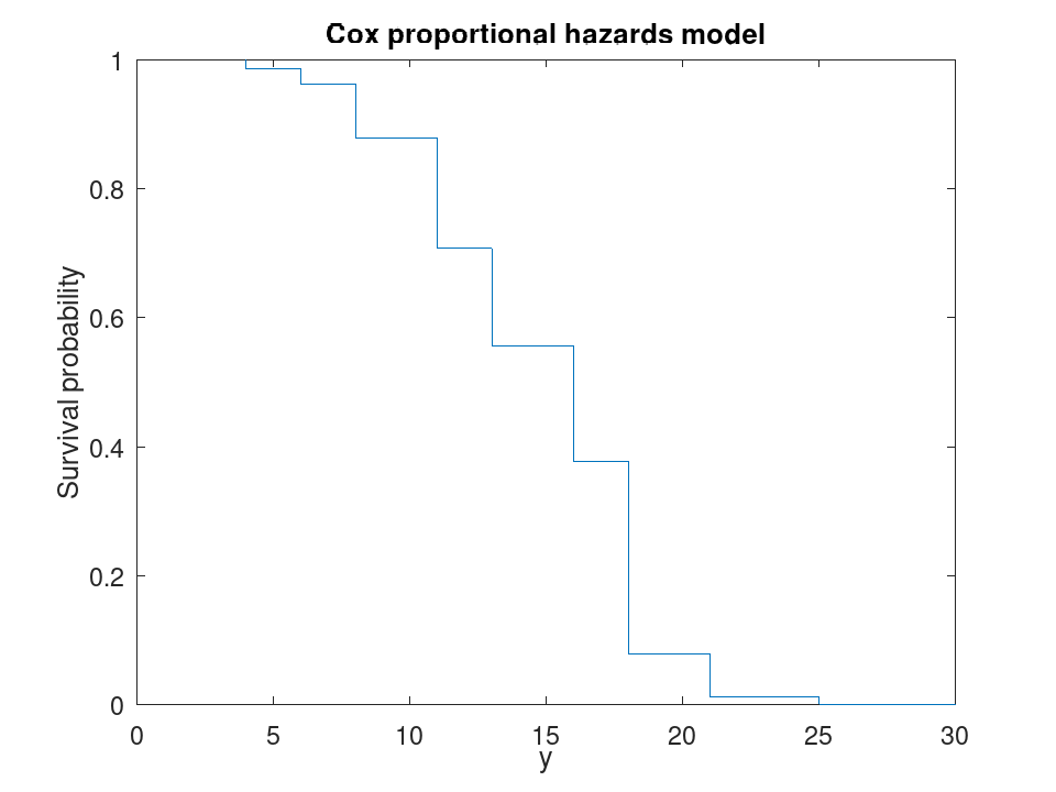
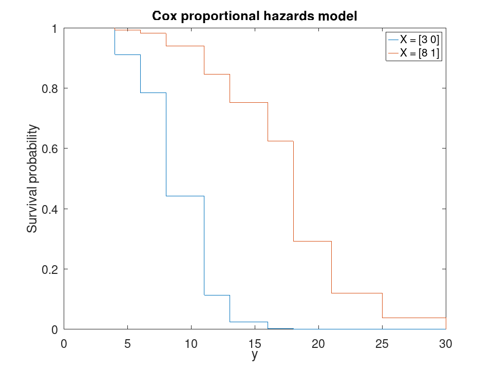
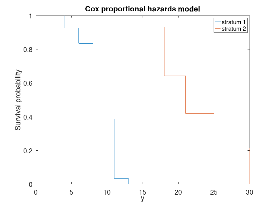
plotSurvival (obj) draws the survival function at the model’s baseline as a stairstep plot. plotSurvival (obj, X) draws it at the predictor values X, one curve per row, and S gives the stratum of each row when the model is stratified. A stratified model with no X draws one curve per stratum.

h = plotSurvival (…) returns the handles of the stairstep lines.

The survival curve of an average observation

 X = [2 0; 5 1; 3 0; 8 1; 4 0; 7 1; 6 0; 9 1; 5 0; 10 1];
 T = [4; 6; 8; 11; 13; 16; 18; 21; 25; 30];
 mdl = fitcox (X, T);

The curve steps down at every event time, and nowhere else: the model learns about survival only where something happened

 plotSurvival (mdl);

Comparing two sets of predictor values

 X = [2 0; 5 1; 3 0; 8 1; 4 0; 7 1; 6 0; 9 1; 5 0; 10 1];
 T = [4; 6; 8; 11; 13; 16; 18; 21; 25; 30];
 mdl = fitcox (X, T);

Proportional hazards means the curves are powers of one another, so they cannot cross

 plotSurvival (mdl, [3 0; 8 1]);
 legend ({'X = [3 0]', 'X = [8 1]'});

One curve per stratum

 X = [2 0; 5 1; 3 0; 8 1; 4 0; 7 1; 6 0; 9 1; 5 0; 10 1];
 T = [4; 6; 8; 11; 13; 16; 18; 21; 25; 30];
 S = [1; 1; 1; 1; 1; 2; 2; 2; 2; 2];
 mdl = fitcox (X, T, 'Stratification', S);

Stratification is what to reach for when the baseline hazards differ: these two curves are under no obligation to be proportional

 plotSurvival (mdl);
 legend ({'stratum 1', 'stratum 2'});

CoxModel: s = survival (obj)
CoxModel: s = survival (obj, X)
CoxModel: s = survival (obj, X, S)
CoxModel: s = survival (…, Name, Value)
CoxModel: [s, T] = survival (…)

s = survival (obj) returns the survival probability at the model’s baseline, evaluated at each row of the Hazard property. s = survival (obj, X) evaluates it at the predictor values X, and S gives the stratum of each row when the model is stratified. For a stratified model s is a cell array holding one column vector per curve.

[s, T] = survival (…) also returns the times the probabilities refer to.

The following Name/Value pairs are accepted:

Name	Value
`"Time"`	The times at which to evaluate the survival function. The default is the model’s own event times. The baseline survival is interpolated linearly between them and raised to the hazard ratio of `X`.
`"ExtrapolationMethod"`	How to evaluate a time outside the model’s event times: `"nearest"` (default), `"linear"`, `"next"`, `"previous"`, or `"none"`. `"none"` returns `NaN` outside the range, as do `"next"` above it and `"previous"` below it.

The survival function at the model's baseline

 X = [2 0; 5 1; 3 0; 8 1; 4 0; 7 1; 6 0; 9 1; 5 0; 10 1];
 T = [4; 6; 8; 11; 13; 16; 18; 21; 25; 30];
 mdl = fitcox (X, T);

Without predictor values the curve is that of an average observation

 [s, t] = survival (mdl);
 table (t, s, 'VariableNames', {'Time', 'Survival'})

ans =
  11x2 table

    Time     Survival      
    ____    ___________    

       4              1    
       4       0.985241    
       6       0.962116    
       8       0.877785    
      11       0.707219    
      13       0.555594    
      16       0.377049    
      18      0.0787367    
      21      0.0124051    
      25      0.0011494    
      30    4.38038e-18

One curve per observation

 X = [2 0; 5 1; 3 0; 8 1; 4 0; 7 1; 6 0; 9 1; 5 0; 10 1];
 T = [4; 6; 8; 11; 13; 16; 18; 21; 25; 30];
 mdl = fitcox (X, T);

The columns follow the rows of X, all on the one grid of event times

 s = survival (mdl, X(1:3,:));
 size (s)

ans =

   11    3

 s(1:4,:)

ans =

   1.000000   1.000000   1.000000
   0.688004   0.628798   0.910944
   0.378589   0.299684   0.784848
   0.037690   0.017125   0.441447

Survival at times of your own

 X = [2 0; 5 1; 3 0; 8 1; 4 0; 7 1; 6 0; 9 1; 5 0; 10 1];
 T = [4; 6; 8; 11; 13; 16; 18; 21; 25; 30];
 mdl = fitcox (X, T);

The baseline survival is interpolated linearly between the event times and then raised to the hazard ratio of the given predictors

 survival (mdl, X(1,:), 'Time', [5; 12; 20])

ans =

   5.1127e-01
   9.5015e-06
   1.7031e-37

Outside the event times the extrapolation rule decides

 X = [2 0; 5 1; 3 0; 8 1; 4 0; 7 1; 6 0; 9 1; 5 0; 10 1];
 T = [4; 6; 8; 11; 13; 16; 18; 21; 25; 30];
 mdl = fitcox (X, T);

The model knows nothing before t = 4 or after t = 30. 'nearest', the default, carries the end values outward; 'none' refuses to answer

 tq = [1; 15; 40];
 nearest = survival (mdl, 'Time', tq);
 none    = survival (mdl, 'Time', tq, 'ExtrapolationMethod', 'none');
 table (tq, nearest, none)

ans =
  3x3 table

    tq      nearest        none      
    __    ___________    ________    

     1              1         NaN    
    15       0.436564    0.436564    
    40    4.38038e-18         NaN

A stratified model gives each stratum its own curve

 X = [2 0; 5 1; 3 0; 8 1; 4 0; 7 1; 6 0; 9 1; 5 0; 10 1];
 T = [4; 6; 8; 11; 13; 16; 18; 21; 25; 30];
 S = [1; 1; 1; 1; 1; 2; 2; 2; 2; 2];
 mdl = fitcox (X, T, 'Stratification', S);

Each stratum carries its own baseline hazard, so the curves are returned separately, on their own event times

 [s, t] = survival (mdl);
 [t{1}, s{1}]

ans =

   4.0000e+00   1.0000e+00
   4.0000e+00   9.2567e-01
   6.0000e+00   8.3461e-01
   8.0000e+00   3.8775e-01
   1.1000e+01   3.3930e-02
   1.3000e+01   5.5295e-04

 [t{2}, s{2}]

ans =

   1.6000e+01   1.0000e+00
   1.6000e+01   9.3273e-01
   1.8000e+01   6.4272e-01
   2.1000e+01   4.1964e-01
   2.5000e+01   2.1387e-01
   3.0000e+01   2.9932e-03

Examples

 X = [2 0; 5 1; 3 0; 8 1; 4 0; 7 1; 6 0; 9 1; 5 0; 10 1];
 T = [4; 6; 8; 11; 13; 16; 18; 21; 25; 30];
 mdl = fitcox (X, T)

mdl =

  Cox proportional hazards regression model:
      y ~ X1 + X2

  Coefficients:

  2x4 table

            Beta         SE        zStat       pValue      
          ________    ________    ________    _________    

    X1    -1.38861    0.527378    -2.63305    0.0084623    
    X2     4.38144     1.85374     2.36357    0.0180998    


Log-likelihood: -8.80696
Likelihood ratio test vs. constant model: p-value = 0.001841

 X = [2 0; 5 1; 3 0; 8 1; 4 0; 7 1; 6 0; 9 1; 5 0; 10 1];
 T = [4; 6; 8; 11; 13; 16; 18; 21; 25; 30];
 mdl = fitcox (X, T);
 [s, t] = survival (mdl);
 [t, s]

ans =

   4.0000e+00   1.0000e+00
   4.0000e+00   9.8524e-01
   6.0000e+00   9.6212e-01
   8.0000e+00   8.7779e-01
   1.1000e+01   7.0722e-01
   1.3000e+01   5.5559e-01
   1.6000e+01   3.7705e-01
   1.8000e+01   7.8737e-02
   2.1000e+01   1.2405e-02
   2.5000e+01   1.1494e-03
   3.0000e+01   4.3804e-18

Categories &

Functions List

Descriptive Statistics

Descriptive Statistics

Data Manipulation

Data Manipulation

Hypothesis Testing

Hypothesis Testing

Experimental Design

Experimental Design

Regression

Regression

Supervised Learning

Supervised Learning

Clustering

Clustering

Nearest Neighbors

Nearest Neighbors

Anomaly Detection

Anomaly Detection

Dimensionality Reduction

Dimensionality Reduction

Model Evaluation

Model Evaluation

Markov Models

Markov Models

Random Sampling

Random Sampling

Distribution Classes

Distribution Classes

Distribution Fitting

Distribution Fitting

Distribution Functions

Distribution Functions

Distribution Statistics

Distribution Statistics

Distribution Wrappers

Distribution Wrappers

Plotting

Plotting

I/O

I/O

Utilities

Utilities

Class Definition: CoxModel

statistics: CoxModel

Coefficients

NumPredictors

LogLikelihood

Hazard

PredictorNames

ResponseName

Formula

Baseline

Stratification

CoefficientCovariance

StandardError

Residuals

ProportionalHazardsPValue

ProportionalHazardsPValueGlobal

LikelihoodRatioTestPValue

VariableInfo

CoxModel

CoxModel: mdl = CoxModel (X, T)

CoxModel: mdl = CoxModel (tbl, respvar)

CoxModel: mdl = CoxModel (…, Name, Value)

coefci

CoxModel: ci = coefci (obj)

CoxModel: ci = coefci (obj, level)

discardResiduals

CoxModel: obj = discardResiduals (obj)

hazardratio

CoxModel: hr = hazardratio (obj, X)

CoxModel: hr = hazardratio (obj, X, S)

CoxModel: hr = hazardratio (…, "Baseline", B)

linhyptest

CoxModel: tbl = linhyptest (obj)

plotSurvival

CoxModel: plotSurvival (obj)

CoxModel: plotSurvival (obj, X)

Class Definition: `CoxModel`

`Coefficients`

`NumPredictors`

`LogLikelihood`

`Hazard`

`PredictorNames`

`ResponseName`

`Formula`

`Baseline`

`Stratification`

`CoefficientCovariance`

`StandardError`

`Residuals`

`ProportionalHazardsPValue`

`ProportionalHazardsPValueGlobal`

`LikelihoodRatioTestPValue`

`VariableInfo`

`CoxModel`

`CoxModel: mdl = CoxModel (X, T)`

`CoxModel: mdl = CoxModel (tbl, respvar)`

`CoxModel: mdl = CoxModel (…, Name, Value)`

`coefci`

`CoxModel: ci = coefci (obj)`

`CoxModel: ci = coefci (obj, level)`

`discardResiduals`

`CoxModel: obj = discardResiduals (obj)`

`hazardratio`

`CoxModel: hr = hazardratio (obj, X)`

`CoxModel: hr = hazardratio (obj, X, S)`

`CoxModel: hr = hazardratio (…, "Baseline", B)`

`linhyptest`

`CoxModel: tbl = linhyptest (obj)`

`plotSurvival`

`CoxModel: plotSurvival (obj)`

`CoxModel: plotSurvival (obj, X)`

`CoxModel: plotSurvival (obj, X, S)`

`CoxModel: h = plotSurvival (…)`

`survival`

`CoxModel: s = survival (obj)`

`CoxModel: s = survival (obj, X)`

`CoxModel: s = survival (obj, X, S)`

`CoxModel: s = survival (…, Name, Value)`

`CoxModel: [s, T] = survival (…)`