Categories &
Functions List
- adtest
- anova
- anova1
- anova2
- anovan
- ansaribradley
- barttest
- binotest
- chi2gof
- chi2test
- correlation_test
- detectdrift
- dwtest
- fishertest
- friedman
- hotelling_t2test
- hotelling_t2test2
- jbtest
- knntest
- kruskalwallis
- kstest
- kstest2
- lillietest
- manova1
- mcnemar_test
- meanEffectSize
- mmdtest
- multcompare
- ranksum
- regression_ftest
- regression_ttest
- runstest
- signrank
- signtest
- stats.drift.DriftDiagnostics
- swtest
- ttest
- ttest2
- vartest
- vartest2
- vartestn
- ztest
- ztest2
- CompactLinearModel
- CoxModel
- coxphfit
- fitcox
- fitglm
- fitglme
- fitlm
- fitlme
- fitlmematrix
- fitnlm
- fitrm
- GeneralizedLinearMixedModel
- GeneralizedLinearModel
- glmfit
- glmval
- invpred
- lasso
- lassoglm
- LinearFormula
- LinearMixedModel
- LinearModel
- logistic_regression
- mnrfit
- mnrval
- monotone_smooth
- mvregress
- mvregresslike
- nlinfit
- nlparci
- nlpredci
- NonLinearModel
- plsregress
- regress
- regress_gp
- RepeatedMeasuresModel
- ridge
- robustfit
- stepwisefit
- stepwiseglm
- stepwiselm
- ClassificationBaggedEnsemble
- ClassificationDiscriminant
- ClassificationECOC
- ClassificationEnsemble
- ClassificationGAM
- ClassificationKernel
- ClassificationKNN
- ClassificationLinear
- ClassificationNaiveBayes
- ClassificationNeuralNetwork
- ClassificationPartitionedECOC
- ClassificationPartitionedEnsemble
- ClassificationPartitionedKernel
- ClassificationPartitionedLinear
- ClassificationPartitionedModel
- ClassificationSVM
- ClassificationTree
- CompactClassificationDiscriminant
- CompactClassificationECOC
- CompactClassificationEnsemble
- CompactClassificationGAM
- CompactClassificationNaiveBayes
- CompactClassificationNeuralNetwork
- CompactClassificationSVM
- CompactClassificationTree
- CompactRegressionGAM
- CompactRegressionEnsemble
- CompactRegressionGP
- CompactRegressionNeuralNetwork
- CompactRegressionSVM
- CompactRegressionTree
- CompactTreeBagger
- designecoc
- fcnnpredict
- fcnntrain
- fitcdiscr
- fitcecoc
- fitcensemble
- fitcgam
- fitckernel
- fitcknn
- fitclinear
- fitcnb
- fitcnet
- fitcsvm
- fitctree
- fitrensemble
- fitrgam
- fitrgp
- fitrkernel
- fitrlinear
- fitrnet
- fitrsvm
- fitrtree
- gamboostinter
- gamboostpairs
- gamboostpredict
- gamboosttrain
- gampredict
- gamtrain
- partialDependence
- plotPartialDependence
- PredictiveModel
- RegressionBaggedEnsemble
- RegressionEnsemble
- RegressionGAM
- RegressionGP
- RegressionKernel
- RegressionLinear
- RegressionNeuralNetwork
- RegressionPartitionedEnsemble
- RegressionPartitionedKernel
- RegressionPartitionedLinear
- RegressionPartitionedModel
- RegressionSVM
- RegressionTree
- lime
- shapley
- svmpredict
- svmtrain
- templateDiscriminant
- templateEnsemble
- templateKernel
- templateKNN
- templateLinear
- templateNaiveBayes
- templateSVM
- templateTree
- TreeBagger
- treepredict
- treetrain
- paretotails
- prob.ProbabilityDistribution
- prob.BetaDistribution
- prob.BinomialDistribution
- prob.BirnbaumSaundersDistribution
- prob.BurrDistribution
- prob.ExponentialDistribution
- prob.ExtremeValueDistribution
- prob.GammaDistribution
- prob.GeneralizedExtremeValueDistribution
- prob.GeneralizedParetoDistribution
- prob.HalfNormalDistribution
- prob.InverseGaussianDistribution
- prob.KernelDistribution
- prob.LogisticDistribution
- prob.LoglogisticDistribution
- prob.LognormalDistribution
- prob.LoguniformDistribution
- prob.MultinomialDistribution
- prob.NakagamiDistribution
- prob.NegativeBinomialDistribution
- prob.NormalDistribution
- prob.PiecewiseLinearDistribution
- prob.PoissonDistribution
- prob.RayleighDistribution
- prob.RicianDistribution
- prob.StableDistribution
- prob.tLocationScaleDistribution
- prob.TriangularDistribution
- prob.UniformDistribution
- prob.WeibullDistribution
- betafit
- betalike
- binofit
- binolike
- bisafit
- bisalike
- burrfit
- burrlike
- copulafit
- evfit
- evlike
- expfit
- explike
- gamfit
- gamlike
- geofit
- gevfit
- gevlike
- gevfit_lmom
- gpfit
- gplike
- gumbelfit
- gumbellike
- hnfit
- hnlike
- invgfit
- invglike
- logifit
- logilike
- loglfit
- logllike
- lognfit
- lognlike
- nakafit
- nakalike
- nbinfit
- nbinlike
- normfit
- normlike
- poissfit
- poisslike
- raylfit
- rayllike
- ricefit
- ricelike
- stblfit
- stbllike
- tlsfit
- tlslike
- unidfit
- unifit
- wblfit
- wbllike
- betacdf
- betainv
- betapdf
- betarnd
- binocdf
- binoinv
- binopdf
- binornd
- bisacdf
- bisainv
- bisapdf
- bisarnd
- burrcdf
- burrinv
- burrpdf
- burrrnd
- bvncdf
- bvtcdf
- cauchycdf
- cauchyinv
- cauchypdf
- cauchyrnd
- chi2cdf
- chi2inv
- chi2pdf
- chi2rnd
- copulacdf
- copulapdf
- copularnd
- evcdf
- evinv
- evpdf
- evrnd
- expcdf
- expinv
- exppdf
- exprnd
- fcdf
- finv
- fpdf
- frnd
- gamcdf
- gaminv
- gampdf
- gamrnd
- geocdf
- geoinv
- geopdf
- geornd
- gevcdf
- gevinv
- gevpdf
- gevrnd
- gpcdf
- gpinv
- gppdf
- gprnd
- gumbelcdf
- gumbelinv
- gumbelpdf
- gumbelrnd
- hncdf
- hninv
- hnpdf
- hnrnd
- hygecdf
- hygeinv
- hygepdf
- hygernd
- invgcdf
- invginv
- invgpdf
- invgrnd
- iwishpdf
- iwishrnd
- jsucdf
- jsupdf
- laplacecdf
- laplaceinv
- laplacepdf
- laplacernd
- logicdf
- logiinv
- logipdf
- logirnd
- loglcdf
- loglinv
- loglpdf
- loglrnd
- logncdf
- logninv
- lognpdf
- lognrnd
- mnpdf
- mnrnd
- mvncdf
- mvnpdf
- mvnrnd
- mvtcdf
- mvtpdf
- mvtrnd
- nakacdf
- nakainv
- nakapdf
- nakarnd
- nbincdf
- nbininv
- nbinpdf
- nbinrnd
- ncfcdf
- ncfinv
- ncfpdf
- ncfrnd
- nctcdf
- nctinv
- nctpdf
- nctrnd
- ncx2cdf
- ncx2inv
- ncx2pdf
- ncx2rnd
- normcdf
- norminv
- normpdf
- normrnd
- plcdf
- plinv
- plpdf
- plrnd
- poisscdf
- poissinv
- poisspdf
- poissrnd
- raylcdf
- raylinv
- raylpdf
- raylrnd
- ricecdf
- riceinv
- ricepdf
- ricernd
- stblcdf
- stblinv
- stblpdf
- stblrnd
- stdrcdf
- stdrinv
- stdrpdf
- stdrrnd
- tcdf
- tinv
- tpdf
- trnd
- tlscdf
- tlsinv
- tlspdf
- tlsrnd
- tricdf
- triinv
- tripdf
- trirnd
- unidcdf
- unidinv
- unidpdf
- unidrnd
- unifcdf
- unifinv
- unifpdf
- unifrnd
- vmcdf
- vminv
- vmpdf
- vmrnd
- wblcdf
- wblinv
- wblpdf
- wblrnd
- wienrnd
- wishpdf
- wishrnd
- betastat
- binostat
- bisastat
- burrstat
- chi2stat
- copulaparam
- copulastat
- evstat
- expstat
- fstat
- gamstat
- geostat
- gevstat
- gpstat
- gumbelstat
- hnstat
- hygestat
- invgstat
- logistat
- loglstat
- lognstat
- nakastat
- nbinstat
- ncfstat
- nctstat
- ncx2stat
- normstat
- plstat
- poisstat
- raylstat
- ricestat
- stdrstat
- tlsstat
- tristat
- tstat
- unidstat
- unifstat
- wblstat
- andrewsplot
- bar3
- bar3h
- biplot
- boxchart
- boxplot
- cdfplot
- dendrogram
- ecdfhist
- einstein
- gardnerAltmanPlot
- glyphplot
- gplotmatrix
- gscatter
- heatmap
- hist3
- histfit
- manovacluster
- normplot
- parallelcoords
- parallelplot
- ppplot
- probplot
- qqplot
- scatterhist
- scatterhistogram
- silhouette
- stats.chart.BoxChart
- stats.chart.HeatmapChart
- stats.chart.ParallelCoordinatesPlot
- stats.chart.ScatterHistogramChart
- swarmchart
- violin
- wblplot
Class Definition: lime
statistics: lime
Local interpretable model-agnostic explanations for a fitted model.
A lime object explains one prediction by fitting a simple model,
a linear one or a shallow decision tree, over observations drawn around
the query point and weighted by how near they lie to it. The simple
model is readable where the fitted one is not, and it is accurate near
the query point rather than everywhere.
explainer = lime (Mdl) builds an explainer for the
fitted model Mdl over the observations it was fitted on. A compact
model keeps none, so it must be given them as X, and so must a
function handle. The observations to fit the simple model on are drawn
at once, and nothing is explained until a query point is given, either to
the constructor as 'QueryPoint' or afterwards to fit.
explainer = lime (Mdl, X) takes the observations
the draw is fitted to as X, a real numeric matrix of one column per
predictor.
X may also be a table, and so may 'QueryPoint',
'CustomSyntheticData' and what fit is given. Where the
model names its predictors the table is read by those names and not by
the order its columns come in, so a column the model was not fitted on is
passed over and a value holding a level is coded as that level was coded
at fitting. A function handle names nothing, so a table given for one
names the predictors itself and its columns are taken in the order they
come.
explainer = lime (fun, X) takes a function
handle in place of a model. fun is called with a matrix of
observations and answers with one column holding one value for each, and
'Type' must say whether those values are a response or a label.
| Name | Value | |
|---|---|---|
'Type' | Whether the model answers with a response,
'regression', or with a label, 'classification'. It is
taken from a fitted model and is required for a function handle. | |
'DataLocality' | Where the observations are drawn
from: 'global', the default, fits the distribution to the whole
of X; 'local' fits it to the 'NumNeighbors'
observations nearest the query point, which must then be known. | |
'NumNeighbors' | How many neighbours
'local' fits to, 1500 by default. | |
'NumSyntheticData' | How many observations to draw, 5000 by default. | |
'CustomSyntheticData' | Observations to use instead of drawing any, one row each. Nothing is drawn where it is given. | |
'CategoricalPredictors' | The predictors whose values are levels, taken as by every learner of this package. It applies only to a function handle, a model being asked for its own. | |
'QueryPoint' | The observation to explain. Given
with 'NumImportantPredictors' it is explained at once, otherwise
it is left to fit. | |
'NumImportantPredictors' | How many predictors the simple model is fitted on. |
Every option fit takes may also be given here, in which case it
stands as the default for every later fit.
'UseParallel' is not implemented and is refused rather than
ignored.
See also: shapley, partialDependence, PredictiveModel
Source Code: lime
The lime class contains the following properties:
The fitted model, or the function handle, the explainer was built on. This property is read-only.
Explain a model fitted from a table
 load fisheriris
 T = table (meas(:,2), meas(:,3), meas(:,4), meas(:,1), ...
            'VariableNames', {'SW', 'PL', 'PW', 'SL'});
 T.Wide = categorical (meas(:,2) > 3, [false true], {'narrow', 'wide'});
 Mdl = fitrtree (T, 'SL');
The observations and the query point may be tables too, read by the names the model was fitted on rather than by the order of the columns
 ex = lime (Mdl, T(:, [1, 2, 3, 5]), 'NumSyntheticData', 2000, ...
            'QueryPoint', T(1, [5, 3, 2, 1]), 'NumImportantPredictors', 2);
 ex.ImportantPredictors'
ans =

   1   2
ex.SimpleModel.Beta'
ans =

   0.2933   0.4740
A column the model was not fitted on is passed over, so the whole table, response and all, may be handed over as it stands
 ex2 = fit (ex, T(1,:), 2);
 ex2.ImportantPredictors'
ans =

   1   2
'global' where the distribution was fitted to the whole of
X, 'local' where it was fitted to the neighbours of
the query point. This property is read-only.
Explain a model fitted from a table
 load fisheriris
 T = table (meas(:,2), meas(:,3), meas(:,4), meas(:,1), ...
            'VariableNames', {'SW', 'PL', 'PW', 'SL'});
 T.Wide = categorical (meas(:,2) > 3, [false true], {'narrow', 'wide'});
 Mdl = fitrtree (T, 'SL');
The observations and the query point may be tables too, read by the names the model was fitted on rather than by the order of the columns
 ex = lime (Mdl, T(:, [1, 2, 3, 5]), 'NumSyntheticData', 2000, ...
            'QueryPoint', T(1, [5, 3, 2, 1]), 'NumImportantPredictors', 2);
 ex.ImportantPredictors'
ans =

   1   2
ex.SimpleModel.Beta'
ans =

   0.2629   0.4658
A column the model was not fitted on is passed over, so the whole table, response and all, may be handed over as it stands
 ex2 = fit (ex, T(1,:), 2);
 ex2.ImportantPredictors'
ans =

   1   2
The indices of the predictors whose values are levels, empty where there are none. This property is read-only.
Explain a model fitted from a table
 load fisheriris
 T = table (meas(:,2), meas(:,3), meas(:,4), meas(:,1), ...
            'VariableNames', {'SW', 'PL', 'PW', 'SL'});
 T.Wide = categorical (meas(:,2) > 3, [false true], {'narrow', 'wide'});
 Mdl = fitrtree (T, 'SL');
The observations and the query point may be tables too, read by the names the model was fitted on rather than by the order of the columns
 ex = lime (Mdl, T(:, [1, 2, 3, 5]), 'NumSyntheticData', 2000, ...
            'QueryPoint', T(1, [5, 3, 2, 1]), 'NumImportantPredictors', 2);
 ex.ImportantPredictors'
ans =

   1   2
ex.SimpleModel.Beta'
ans =

   0.2694   0.4515
A column the model was not fitted on is passed over, so the whole table, response and all, may be handed over as it stands
 ex2 = fit (ex, T(1,:), 2);
 ex2.ImportantPredictors'
ans =

   1   2
'regression' or 'classification'. This property is
read-only.
Explain a model fitted from a table
 load fisheriris
 T = table (meas(:,2), meas(:,3), meas(:,4), meas(:,1), ...
            'VariableNames', {'SW', 'PL', 'PW', 'SL'});
 T.Wide = categorical (meas(:,2) > 3, [false true], {'narrow', 'wide'});
 Mdl = fitrtree (T, 'SL');
The observations and the query point may be tables too, read by the names the model was fitted on rather than by the order of the columns
 ex = lime (Mdl, T(:, [1, 2, 3, 5]), 'NumSyntheticData', 2000, ...
            'QueryPoint', T(1, [5, 3, 2, 1]), 'NumImportantPredictors', 2);
 ex.ImportantPredictors'
ans =

   1   2
ex.SimpleModel.Beta'
ans =

   0.2686   0.4607
A column the model was not fitted on is passed over, so the whole table, response and all, may be handed over as it stands
 ex2 = fit (ex, T(1,:), 2);
 ex2.ImportantPredictors'
ans =

   1   2
A real numeric matrix of one row per observation and one column per predictor. This property is read-only.
Where the observations were given as a table, they are the coded matrix and not the table: a variable holding levels is stored as its level codes, and the coding is kept with the object.
Explain a model fitted from a table
 load fisheriris
 T = table (meas(:,2), meas(:,3), meas(:,4), meas(:,1), ...
            'VariableNames', {'SW', 'PL', 'PW', 'SL'});
 T.Wide = categorical (meas(:,2) > 3, [false true], {'narrow', 'wide'});
 Mdl = fitrtree (T, 'SL');
The observations and the query point may be tables too, read by the names the model was fitted on rather than by the order of the columns
 ex = lime (Mdl, T(:, [1, 2, 3, 5]), 'NumSyntheticData', 2000, ...
            'QueryPoint', T(1, [5, 3, 2, 1]), 'NumImportantPredictors', 2);
 ex.ImportantPredictors'
ans =

   1   2
ex.SimpleModel.Beta'
ans =

   0.2674   0.4604
A column the model was not fitted on is passed over, so the whole table, response and all, may be handed over as it stands
 ex2 = fit (ex, T(1,:), 2);
 ex2.ImportantPredictors'
ans =

   1   2
One row holding one value per predictor, empty until a query point is given. This property is read-only.
Explain a model fitted from a table
 load fisheriris
 T = table (meas(:,2), meas(:,3), meas(:,4), meas(:,1), ...
            'VariableNames', {'SW', 'PL', 'PW', 'SL'});
 T.Wide = categorical (meas(:,2) > 3, [false true], {'narrow', 'wide'});
 Mdl = fitrtree (T, 'SL');
The observations and the query point may be tables too, read by the names the model was fitted on rather than by the order of the columns
 ex = lime (Mdl, T(:, [1, 2, 3, 5]), 'NumSyntheticData', 2000, ...
            'QueryPoint', T(1, [5, 3, 2, 1]), 'NumImportantPredictors', 2);
 ex.ImportantPredictors'
ans =

   1   2
ex.SimpleModel.Beta'
ans =

   0.2432   0.4681
A column the model was not fitted on is passed over, so the whole table, response and all, may be handed over as it stands
 ex2 = fit (ex, T(1,:), 2);
 ex2.ImportantPredictors'
ans =

   1   2
Empty until a query point is given. Fewer may be used, where a predictor adds nothing. This property is read-only.
Explain a model fitted from a table
 load fisheriris
 T = table (meas(:,2), meas(:,3), meas(:,4), meas(:,1), ...
            'VariableNames', {'SW', 'PL', 'PW', 'SL'});
 T.Wide = categorical (meas(:,2) > 3, [false true], {'narrow', 'wide'});
 Mdl = fitrtree (T, 'SL');
The observations and the query point may be tables too, read by the names the model was fitted on rather than by the order of the columns
 ex = lime (Mdl, T(:, [1, 2, 3, 5]), 'NumSyntheticData', 2000, ...
            'QueryPoint', T(1, [5, 3, 2, 1]), 'NumImportantPredictors', 2);
 ex.ImportantPredictors'
ans =

   1   2
ex.SimpleModel.Beta'
ans =

   0.2878   0.4595
A column the model was not fitted on is passed over, so the whole table, response and all, may be handed over as it stands
 ex2 = fit (ex, T(1,:), 2);
 ex2.ImportantPredictors'
ans =

   1   2
This property is read-only.
Explain a model fitted from a table
 load fisheriris
 T = table (meas(:,2), meas(:,3), meas(:,4), meas(:,1), ...
            'VariableNames', {'SW', 'PL', 'PW', 'SL'});
 T.Wide = categorical (meas(:,2) > 3, [false true], {'narrow', 'wide'});
 Mdl = fitrtree (T, 'SL');
The observations and the query point may be tables too, read by the names the model was fitted on rather than by the order of the columns
 ex = lime (Mdl, T(:, [1, 2, 3, 5]), 'NumSyntheticData', 2000, ...
            'QueryPoint', T(1, [5, 3, 2, 1]), 'NumImportantPredictors', 2);
 ex.ImportantPredictors'
ans =

   1   2
ex.SimpleModel.Beta'
ans =

   0.3320   0.4566
A column the model was not fitted on is passed over, so the whole table, response and all, may be handed over as it stands
 ex2 = fit (ex, T(1,:), 2);
 ex2.ImportantPredictors'
ans =

   1   2
One row each, drawn around the query point or given outright as
'CustomSyntheticData'. This property is read-only.
Explain a model fitted from a table
 load fisheriris
 T = table (meas(:,2), meas(:,3), meas(:,4), meas(:,1), ...
            'VariableNames', {'SW', 'PL', 'PW', 'SL'});
 T.Wide = categorical (meas(:,2) > 3, [false true], {'narrow', 'wide'});
 Mdl = fitrtree (T, 'SL');
The observations and the query point may be tables too, read by the names the model was fitted on rather than by the order of the columns
 ex = lime (Mdl, T(:, [1, 2, 3, 5]), 'NumSyntheticData', 2000, ...
            'QueryPoint', T(1, [5, 3, 2, 1]), 'NumImportantPredictors', 2);
 ex.ImportantPredictors'
ans =

   1   2
ex.SimpleModel.Beta'
ans =

   0.3047   0.4677
A column the model was not fitted on is passed over, so the whole table, response and all, may be handed over as it stands
 ex2 = fit (ex, T(1,:), 2);
 ex2.ImportantPredictors'
ans =

   1   2
One response per observation for a regression model, or one label for a classifier, keeping the type of the response the model was fitted with. This property is read-only.
Explain a model fitted from a table
 load fisheriris
 T = table (meas(:,2), meas(:,3), meas(:,4), meas(:,1), ...
            'VariableNames', {'SW', 'PL', 'PW', 'SL'});
 T.Wide = categorical (meas(:,2) > 3, [false true], {'narrow', 'wide'});
 Mdl = fitrtree (T, 'SL');
The observations and the query point may be tables too, read by the names the model was fitted on rather than by the order of the columns
 ex = lime (Mdl, T(:, [1, 2, 3, 5]), 'NumSyntheticData', 2000, ...
            'QueryPoint', T(1, [5, 3, 2, 1]), 'NumImportantPredictors', 2);
 ex.ImportantPredictors'
ans =

   1   2
ex.SimpleModel.Beta'
ans =

   0.2790   0.4772
A column the model was not fitted on is passed over, so the whole table, response and all, may be handed over as it stands
 ex2 = fit (ex, T(1,:), 2);
 ex2.ImportantPredictors'
ans =

   1   2
A RegressionLinear, ClassificationLinear,
RegressionTree or ClassificationTree, fitted on the
important predictors alone and weighted by nearness to the query
point. For a classifier it answers 1 for the class the
explained model predicted and -1 for any other, which is what
makes it a single model however many classes there are. It is empty
until a query point is given. This property is read-only.
Explain a model fitted from a table
 load fisheriris
 T = table (meas(:,2), meas(:,3), meas(:,4), meas(:,1), ...
            'VariableNames', {'SW', 'PL', 'PW', 'SL'});
 T.Wide = categorical (meas(:,2) > 3, [false true], {'narrow', 'wide'});
 Mdl = fitrtree (T, 'SL');
The observations and the query point may be tables too, read by the names the model was fitted on rather than by the order of the columns
 ex = lime (Mdl, T(:, [1, 2, 3, 5]), 'NumSyntheticData', 2000, ...
            'QueryPoint', T(1, [5, 3, 2, 1]), 'NumImportantPredictors', 2);
 ex.ImportantPredictors'
ans =

   1   2
ex.SimpleModel.Beta'
ans =

   0.2416   0.4743
A column the model was not fitted on is passed over, so the whole table, response and all, may be handed over as it stands
 ex2 = fit (ex, T(1,:), 2);
 ex2.ImportantPredictors'
ans =

   1   2
Their indices, in increasing order, empty until a query point is given. This property is read-only.
Explain a model fitted from a table
 load fisheriris
 T = table (meas(:,2), meas(:,3), meas(:,4), meas(:,1), ...
            'VariableNames', {'SW', 'PL', 'PW', 'SL'});
 T.Wide = categorical (meas(:,2) > 3, [false true], {'narrow', 'wide'});
 Mdl = fitrtree (T, 'SL');
The observations and the query point may be tables too, read by the names the model was fitted on rather than by the order of the columns
 ex = lime (Mdl, T(:, [1, 2, 3, 5]), 'NumSyntheticData', 2000, ...
            'QueryPoint', T(1, [5, 3, 2, 1]), 'NumImportantPredictors', 2);
 ex.ImportantPredictors'
ans =

   1   2
ex.SimpleModel.Beta'
ans =

   0.2534   0.4669
A column the model was not fitted on is passed over, so the whole table, response and all, may be handed over as it stands
 ex2 = fit (ex, T(1,:), 2);
 ex2.ImportantPredictors'
ans =

   1   2
This property is read-only.
Explain a model fitted from a table
 load fisheriris
 T = table (meas(:,2), meas(:,3), meas(:,4), meas(:,1), ...
            'VariableNames', {'SW', 'PL', 'PW', 'SL'});
 T.Wide = categorical (meas(:,2) > 3, [false true], {'narrow', 'wide'});
 Mdl = fitrtree (T, 'SL');
The observations and the query point may be tables too, read by the names the model was fitted on rather than by the order of the columns
 ex = lime (Mdl, T(:, [1, 2, 3, 5]), 'NumSyntheticData', 2000, ...
            'QueryPoint', T(1, [5, 3, 2, 1]), 'NumImportantPredictors', 2);
 ex.ImportantPredictors'
ans =

   1   2
ex.SimpleModel.Beta'
ans =

   0.2638   0.4736
A column the model was not fitted on is passed over, so the whole table, response and all, may be handed over as it stands
 ex2 = fit (ex, T(1,:), 2);
 ex2.ImportantPredictors'
ans =

   1   2
Where the two agree the simple model is worth reading; where they do not, it explains nothing. This property is read-only.
Explain a model fitted from a table
 load fisheriris
 T = table (meas(:,2), meas(:,3), meas(:,4), meas(:,1), ...
            'VariableNames', {'SW', 'PL', 'PW', 'SL'});
 T.Wide = categorical (meas(:,2) > 3, [false true], {'narrow', 'wide'});
 Mdl = fitrtree (T, 'SL');
The observations and the query point may be tables too, read by the names the model was fitted on rather than by the order of the columns
 ex = lime (Mdl, T(:, [1, 2, 3, 5]), 'NumSyntheticData', 2000, ...
            'QueryPoint', T(1, [5, 3, 2, 1]), 'NumImportantPredictors', 2);
 ex.ImportantPredictors'
ans =

   1   2
ex.SimpleModel.Beta'
ans =

   0.2378   0.4695
A column the model was not fitted on is passed over, so the whole table, response and all, may be handed over as it stands
 ex2 = fit (ex, T(1,:), 2);
 ex2.ImportantPredictors'
ans =

   1   2
The lime class offers the following public methods:
lime: obj = lime (Mdl)
lime: obj = lime (Mdl, X)
lime: obj = lime (fun, X)
lime: obj = lime (…, name, value)
The arguments are those described for the class. The observations
the simple model is fitted over are drawn here; where
'QueryPoint' and 'NumImportantPredictors' are both
given the explanation is computed at once, otherwise it is left to
fit.
See also: lime, lime.fit, lime.plot
Explain a model fitted from a table
 load fisheriris
 T = table (meas(:,2), meas(:,3), meas(:,4), meas(:,1), ...
            'VariableNames', {'SW', 'PL', 'PW', 'SL'});
 T.Wide = categorical (meas(:,2) > 3, [false true], {'narrow', 'wide'});
 Mdl = fitrtree (T, 'SL');
The observations and the query point may be tables too, read by the names the model was fitted on rather than by the order of the columns
 ex = lime (Mdl, T(:, [1, 2, 3, 5]), 'NumSyntheticData', 2000, ...
            'QueryPoint', T(1, [5, 3, 2, 1]), 'NumImportantPredictors', 2);
 ex.ImportantPredictors'
ans =

   1   2
ex.SimpleModel.Beta'
ans =

   0.3268   0.4566
A column the model was not fitted on is passed over, so the whole table, response and all, may be handed over as it stands
 ex2 = fit (ex, T(1,:), 2);
 ex2.ImportantPredictors'
ans =

   1   2
lime: obj = fit (obj, queryPoint, numImportantPredictors)
lime: obj = fit (…, name, value)
queryPoint is one row holding one value per predictor, or a
table read by the names the explainer holds, and
numImportantPredictors how many predictors the simple model is
fitted on. Fewer are used where a predictor adds nothing, and
ImportantPredictors says which were.
| Name | Value | |
|---|---|---|
'Distance' | How nearness to the query point is
measured. Where the predictors hold numbers it is one of
'euclidean', the default, 'squaredeuclidean',
'seuclidean', 'mahalanobis', 'cityblock',
'minkowski', 'chebychev', 'cosine',
'correlation' and 'spearman'; where some hold levels
it is 'goodall3', the default, or 'ofd'. Both count
level frequencies over the drawn observations and the query point
together. 'goodall3' is the 'goodall3' measure of
nomdist; 'ofd' is one less the mean similarity of its
'of' measure, D / (1 + D) of the D it returns.
A function handle is also taken, which MATLAB does not; see below. | |
'KernelWidth' | How sharply the weight falls away with distance, from just above 0 to 1. The default is 0.75. | |
'SimpleModelType' | 'linear', the
default, or 'tree'. | |
'BetaTolerance' | Relative tolerance the linear simple model is fitted to, 10^{-4} by default. | |
'Cov', 'P', 'Scale' | Passed to
the distance that takes them, as pdist2 takes them. |
The weight of a drawn observation is
exp (-0.5 (d / D / w)^2), with d its distance from the
query point and w the kernel width. D is the square
root of the number of predictors for 'goodall3' and
'ofd', and otherwise the largest distance between two drawn
observations.
A predictor holding levels enters a linear simple model as one column for each level other than the query point’s, saying whether an observation holds that level, so each coefficient is read against the query point’s level.
Where the predictors mix numbers and levels, 'goodall3' and
'ofd' score a predictor holding numbers by one less its
absolute difference over its range, the query point included, and
average that with the similarities of the predictors holding levels.
MATLAB does so by a rule it does not document, which none of the
constructions tried here reproduces, so on such data the explanation
differs from MATLAB’s. On levels alone 'goodall3' agrees with
MATLAB; MATLAB does not document 'ofd' beyond scoring a match
0, and its coefficients differ from those here by up to 0.006
on the fixture measured.
- Explaining one prediction with a simple model
 load fisheriris
 mdl = fitrtree (meas(:,2:4), meas(:,1));
 ex = lime (mdl, 'NumSyntheticData', 2000);
The explainer draws its observations when it is built, and explains nothing until a query point is given
ex = fit (ex, meas(1,2:4), 2);
The two predictors the simple model was fitted on, and its weights
ex.ImportantPredictors'
ans =

   1   2
ex.SimpleModel.Beta'
ans =

   0.2977   0.4823
- Reading whether the explanation is worth trusting
 load fisheriris
 mdl = fitrtree (meas(:,2:4), meas(:,1));
 ex = fit (lime (mdl, 'NumSyntheticData', 2000), meas(1,2:4), 3);
A simple model that answers near what the explained model answered is worth reading; one that does not explains nothing
[ex.BlackboxFitted, ex.SimpleModelFitted]
ans =

   5.0333   4.7520
- Drawing near the query point rather than over everything
 load fisheriris
 mdl = fitrtree (meas(:,2:4), meas(:,1));
'local' fits the draw to the neighbours of the query point, so the simple model sees the shape of the model there rather than everywhere
 ex = lime (mdl, 'DataLocality', 'local', 'NumNeighbors', 30, ...
            'NumSyntheticData', 2000, 'QueryPoint', meas(1,2:4), ...
            'NumImportantPredictors', 2);
 ex.ImportantPredictors'
ans =

   1   3
ex.SimpleModel.Beta'
ans =

   0.6966  -0.2980
- A tree in place of the weighted sum
 load fisheriris
 mdl = fitcknn (meas, species);
 ex = lime (mdl, 'NumSyntheticData', 2000);
A classifier is explained one class at a time: the simple model separates the class the explained model predicted from every other, answering 1 for it and -1 for the rest
 ex = fit (ex, meas(1,:), 2, 'SimpleModelType', 'tree');
 class (ex.SimpleModel)
ans = ClassificationTree
ex.BlackboxFitted
ans =
  1x1 cell array

    {'setosa'}
ex.SimpleModelFitted
ans = 1
lime: plot (obj)
lime: f = plot (obj)
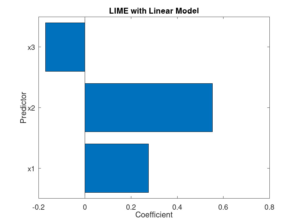
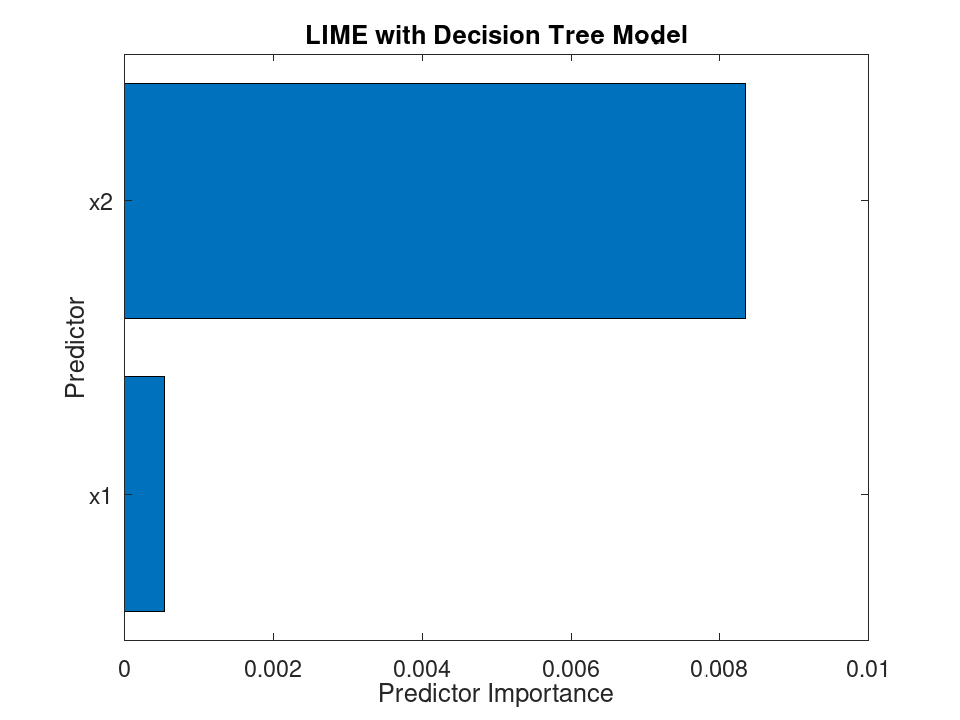
A horizontal bar per important predictor, holding the coefficient of a linear simple model or the predictor importance of a tree, in the order the predictors come in rather than by size. f is the figure drawn.
- What the simple model says about the query point
 load fisheriris
 mdl = fitrtree (meas(:,2:4), meas(:,1));
 ex = fit (lime (mdl, 'NumSyntheticData', 2000), meas(1,2:4), 3);
One bar per predictor the simple model was fitted on, holding its weight, so a long bar is a predictor the prediction turns on here
plot (ex);
- A narrower explanation
 load fisheriris
 mdl = fitrtree (meas(:,2:4), meas(:,1));
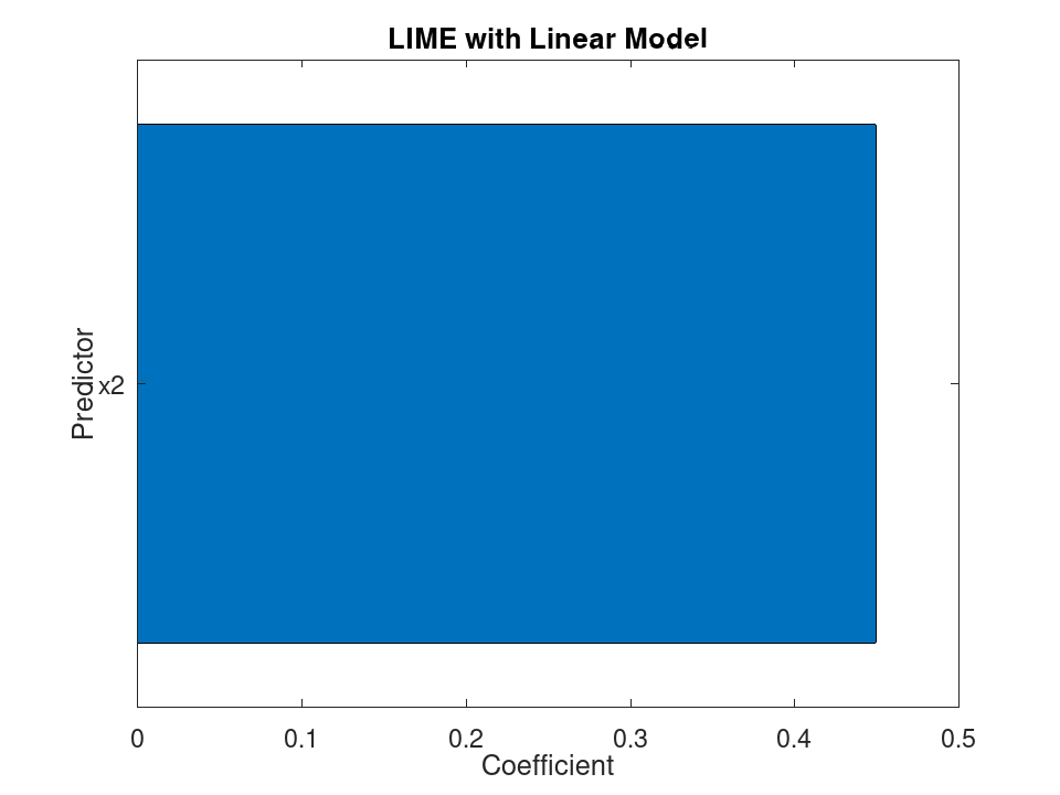
Asking for fewer predictors gives a simple model that is easier to read and further from the one it explains
 ex = fit (lime (mdl, 'NumSyntheticData', 2000), meas(1,2:4), 1);
 plot (ex);
- A tree is drawn by what it splits on
 load fisheriris
 mdl = fitrtree (meas(:,2:4), meas(:,1));
 ex = fit (lime (mdl, 'NumSyntheticData', 2000), meas(1,2:4), 2, ...
           'SimpleModelType', 'tree');
A tree has no weights to show, so the bars hold predictor importance and the chart is titled after what the simple model is
plot (ex);
Examples
 load fisheriris
 T = table (meas(:,2), meas(:,3), meas(:,4), meas(:,1), ...
            'VariableNames', {'SW', 'PL', 'PW', 'SL'});
 T.Wide = categorical (meas(:,2) > 3, [false true], {'narrow', 'wide'});
 Mdl = fitrtree (T, 'SL');
The observations and the query point may be tables too, read by the names the model was fitted on rather than by the order of the columns
 ex = lime (Mdl, T(:, [1, 2, 3, 5]), 'NumSyntheticData', 2000, ...
            'QueryPoint', T(1, [5, 3, 2, 1]), 'NumImportantPredictors', 2);
 ex.ImportantPredictors'
ans =

   1   2
ex.SimpleModel.Beta'
ans =

   0.3108   0.4580
A column the model was not fitted on is passed over, so the whole table, response and all, may be handed over as it stands
 ex2 = fit (ex, T(1,:), 2);
 ex2.ImportantPredictors'
ans =

   1   2