Categories &
Functions List
- adtest
- anova
- anova1
- anova2
- anovan
- ansaribradley
- barttest
- binotest
- chi2gof
- chi2test
- correlation_test
- detectdrift
- dwtest
- fishertest
- friedman
- hotelling_t2test
- hotelling_t2test2
- jbtest
- knntest
- kruskalwallis
- kstest
- kstest2
- lillietest
- manova1
- mcnemar_test
- meanEffectSize
- mmdtest
- multcompare
- ranksum
- regression_ftest
- regression_ttest
- runstest
- signrank
- signtest
- stats.drift.DriftDiagnostics
- swtest
- ttest
- ttest2
- vartest
- vartest2
- vartestn
- ztest
- ztest2
- CompactLinearModel
- CoxModel
- coxphfit
- fitcox
- fitglm
- fitglme
- fitlm
- fitlme
- fitlmematrix
- fitnlm
- fitrm
- GeneralizedLinearMixedModel
- GeneralizedLinearModel
- glmfit
- glmval
- invpred
- lasso
- lassoglm
- LinearFormula
- LinearMixedModel
- LinearModel
- logistic_regression
- mnrfit
- mnrval
- monotone_smooth
- mvregress
- mvregresslike
- nlinfit
- nlparci
- nlpredci
- NonLinearModel
- plsregress
- regress
- regress_gp
- RepeatedMeasuresModel
- ridge
- robustfit
- stepwisefit
- stepwiseglm
- stepwiselm
- ClassificationBaggedEnsemble
- ClassificationDiscriminant
- ClassificationECOC
- ClassificationEnsemble
- ClassificationGAM
- ClassificationKernel
- ClassificationKNN
- ClassificationLinear
- ClassificationNaiveBayes
- ClassificationNeuralNetwork
- ClassificationPartitionedECOC
- ClassificationPartitionedEnsemble
- ClassificationPartitionedKernel
- ClassificationPartitionedLinear
- ClassificationPartitionedModel
- ClassificationSVM
- ClassificationTree
- CompactClassificationDiscriminant
- CompactClassificationECOC
- CompactClassificationEnsemble
- CompactClassificationGAM
- CompactClassificationNaiveBayes
- CompactClassificationNeuralNetwork
- CompactClassificationSVM
- CompactClassificationTree
- CompactRegressionGAM
- CompactRegressionEnsemble
- CompactRegressionGP
- CompactRegressionNeuralNetwork
- CompactRegressionSVM
- CompactRegressionTree
- CompactTreeBagger
- designecoc
- fcnnpredict
- fcnntrain
- fitcdiscr
- fitcecoc
- fitcensemble
- fitcgam
- fitckernel
- fitcknn
- fitclinear
- fitcnb
- fitcnet
- fitcsvm
- fitctree
- fitrensemble
- fitrgam
- fitrgp
- fitrkernel
- fitrlinear
- fitrnet
- fitrsvm
- fitrtree
- gamboostinter
- gamboostpairs
- gamboostpredict
- gamboosttrain
- gampredict
- gamtrain
- partialDependence
- plotPartialDependence
- PredictiveModel
- RegressionBaggedEnsemble
- RegressionEnsemble
- RegressionGAM
- RegressionGP
- RegressionKernel
- RegressionLinear
- RegressionNeuralNetwork
- RegressionPartitionedEnsemble
- RegressionPartitionedKernel
- RegressionPartitionedLinear
- RegressionPartitionedModel
- RegressionSVM
- RegressionTree
- lime
- shapley
- svmpredict
- svmtrain
- templateDiscriminant
- templateEnsemble
- templateKernel
- templateKNN
- templateLinear
- templateNaiveBayes
- templateSVM
- templateTree
- TreeBagger
- treepredict
- treetrain
- paretotails
- prob.ProbabilityDistribution
- prob.BetaDistribution
- prob.BinomialDistribution
- prob.BirnbaumSaundersDistribution
- prob.BurrDistribution
- prob.ExponentialDistribution
- prob.ExtremeValueDistribution
- prob.GammaDistribution
- prob.GeneralizedExtremeValueDistribution
- prob.GeneralizedParetoDistribution
- prob.HalfNormalDistribution
- prob.InverseGaussianDistribution
- prob.KernelDistribution
- prob.LogisticDistribution
- prob.LoglogisticDistribution
- prob.LognormalDistribution
- prob.LoguniformDistribution
- prob.MultinomialDistribution
- prob.NakagamiDistribution
- prob.NegativeBinomialDistribution
- prob.NormalDistribution
- prob.PiecewiseLinearDistribution
- prob.PoissonDistribution
- prob.RayleighDistribution
- prob.RicianDistribution
- prob.StableDistribution
- prob.tLocationScaleDistribution
- prob.TriangularDistribution
- prob.UniformDistribution
- prob.WeibullDistribution
- betafit
- betalike
- binofit
- binolike
- bisafit
- bisalike
- burrfit
- burrlike
- copulafit
- evfit
- evlike
- expfit
- explike
- gamfit
- gamlike
- geofit
- gevfit
- gevlike
- gevfit_lmom
- gpfit
- gplike
- gumbelfit
- gumbellike
- hnfit
- hnlike
- invgfit
- invglike
- logifit
- logilike
- loglfit
- logllike
- lognfit
- lognlike
- nakafit
- nakalike
- nbinfit
- nbinlike
- normfit
- normlike
- poissfit
- poisslike
- raylfit
- rayllike
- ricefit
- ricelike
- stblfit
- stbllike
- tlsfit
- tlslike
- unidfit
- unifit
- wblfit
- wbllike
- betacdf
- betainv
- betapdf
- betarnd
- binocdf
- binoinv
- binopdf
- binornd
- bisacdf
- bisainv
- bisapdf
- bisarnd
- burrcdf
- burrinv
- burrpdf
- burrrnd
- bvncdf
- bvtcdf
- cauchycdf
- cauchyinv
- cauchypdf
- cauchyrnd
- chi2cdf
- chi2inv
- chi2pdf
- chi2rnd
- copulacdf
- copulapdf
- copularnd
- evcdf
- evinv
- evpdf
- evrnd
- expcdf
- expinv
- exppdf
- exprnd
- fcdf
- finv
- fpdf
- frnd
- gamcdf
- gaminv
- gampdf
- gamrnd
- geocdf
- geoinv
- geopdf
- geornd
- gevcdf
- gevinv
- gevpdf
- gevrnd
- gpcdf
- gpinv
- gppdf
- gprnd
- gumbelcdf
- gumbelinv
- gumbelpdf
- gumbelrnd
- hncdf
- hninv
- hnpdf
- hnrnd
- hygecdf
- hygeinv
- hygepdf
- hygernd
- invgcdf
- invginv
- invgpdf
- invgrnd
- iwishpdf
- iwishrnd
- jsucdf
- jsupdf
- laplacecdf
- laplaceinv
- laplacepdf
- laplacernd
- logicdf
- logiinv
- logipdf
- logirnd
- loglcdf
- loglinv
- loglpdf
- loglrnd
- logncdf
- logninv
- lognpdf
- lognrnd
- mnpdf
- mnrnd
- mvncdf
- mvnpdf
- mvnrnd
- mvtcdf
- mvtpdf
- mvtrnd
- nakacdf
- nakainv
- nakapdf
- nakarnd
- nbincdf
- nbininv
- nbinpdf
- nbinrnd
- ncfcdf
- ncfinv
- ncfpdf
- ncfrnd
- nctcdf
- nctinv
- nctpdf
- nctrnd
- ncx2cdf
- ncx2inv
- ncx2pdf
- ncx2rnd
- normcdf
- norminv
- normpdf
- normrnd
- plcdf
- plinv
- plpdf
- plrnd
- poisscdf
- poissinv
- poisspdf
- poissrnd
- raylcdf
- raylinv
- raylpdf
- raylrnd
- ricecdf
- riceinv
- ricepdf
- ricernd
- stblcdf
- stblinv
- stblpdf
- stblrnd
- stdrcdf
- stdrinv
- stdrpdf
- stdrrnd
- tcdf
- tinv
- tpdf
- trnd
- tlscdf
- tlsinv
- tlspdf
- tlsrnd
- tricdf
- triinv
- tripdf
- trirnd
- unidcdf
- unidinv
- unidpdf
- unidrnd
- unifcdf
- unifinv
- unifpdf
- unifrnd
- vmcdf
- vminv
- vmpdf
- vmrnd
- wblcdf
- wblinv
- wblpdf
- wblrnd
- wienrnd
- wishpdf
- wishrnd
- betastat
- binostat
- bisastat
- burrstat
- chi2stat
- copulaparam
- copulastat
- evstat
- expstat
- fstat
- gamstat
- geostat
- gevstat
- gpstat
- gumbelstat
- hnstat
- hygestat
- invgstat
- logistat
- loglstat
- lognstat
- nakastat
- nbinstat
- ncfstat
- nctstat
- ncx2stat
- normstat
- plstat
- poisstat
- raylstat
- ricestat
- stdrstat
- tlsstat
- tristat
- tstat
- unidstat
- unifstat
- wblstat
- andrewsplot
- bar3
- bar3h
- biplot
- boxchart
- boxplot
- cdfplot
- dendrogram
- ecdfhist
- einstein
- gardnerAltmanPlot
- glyphplot
- gplotmatrix
- gscatter
- heatmap
- hist3
- histfit
- manovacluster
- normplot
- parallelcoords
- parallelplot
- ppplot
- probplot
- qqplot
- scatterhist
- scatterhistogram
- silhouette
- stats.chart.BoxChart
- stats.chart.HeatmapChart
- stats.chart.ParallelCoordinatesPlot
- stats.chart.ScatterHistogramChart
- swarmchart
- violin
- wblplot
Class Definition: RegressionGP
statistics: RegressionGP
Gaussian process regression model.
A RegressionGP object holds a Gaussian process fitted to a
continuous response, and predicts the response for new data with the
predict method, which also returns the standard deviation of each
prediction and a prediction interval. The response is modelled as an
explicit basis times Beta, plus a draw from a process whose
covariance is given by the kernel function, plus independent noise of
standard deviation Sigma. The kernel parameters and Sigma
are estimated by maximizing the log marginal likelihood.
The object keeps its training data, which resubPredict,
resubLoss and crossval work on; compact drops it and
returns a CompactRegressionGP, which still predicts.
Create a RegressionGP object with fitrgp or the class
constructor.
See also: fitrgp, CompactRegressionGP
Source Code: RegressionGP
The RegressionGP class contains the following properties:
An NxP numeric matrix, as it was supplied to the constructor.
Where the model was fitted from a table, the predictors are the coded matrix and not the table: a variable holding levels is stored as its level codes, and the coding is kept with the model.
This property is read-only.
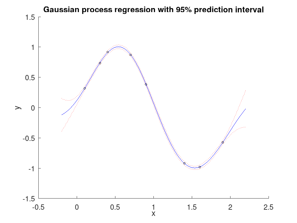
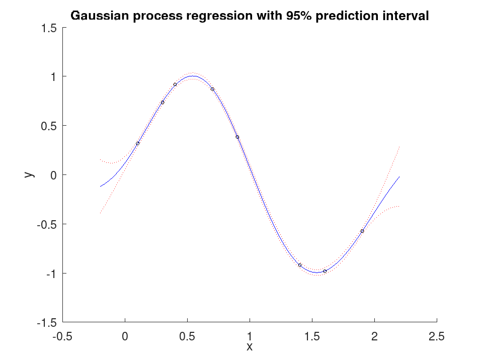
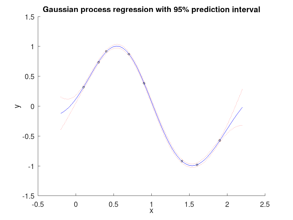
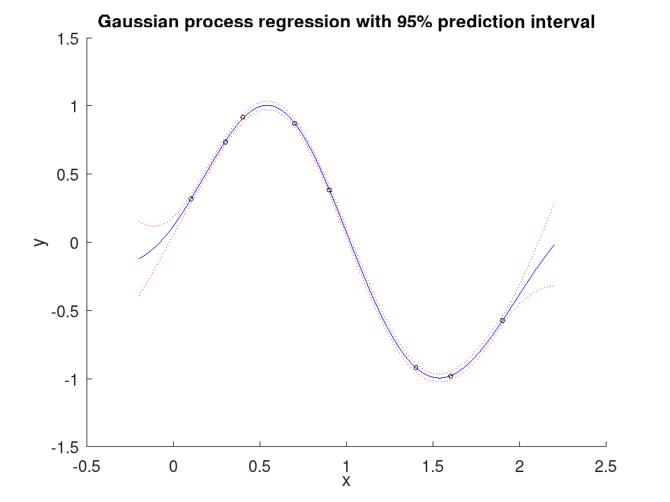
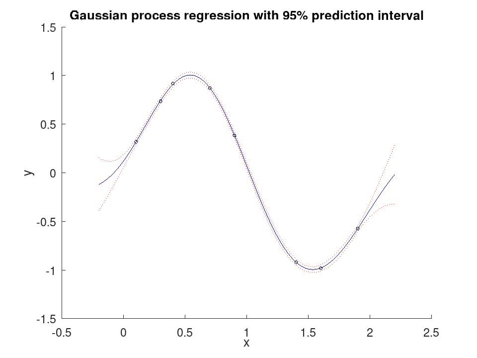
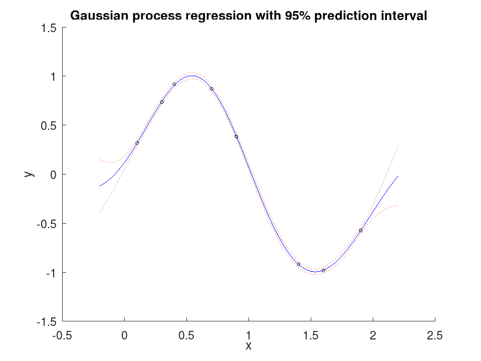
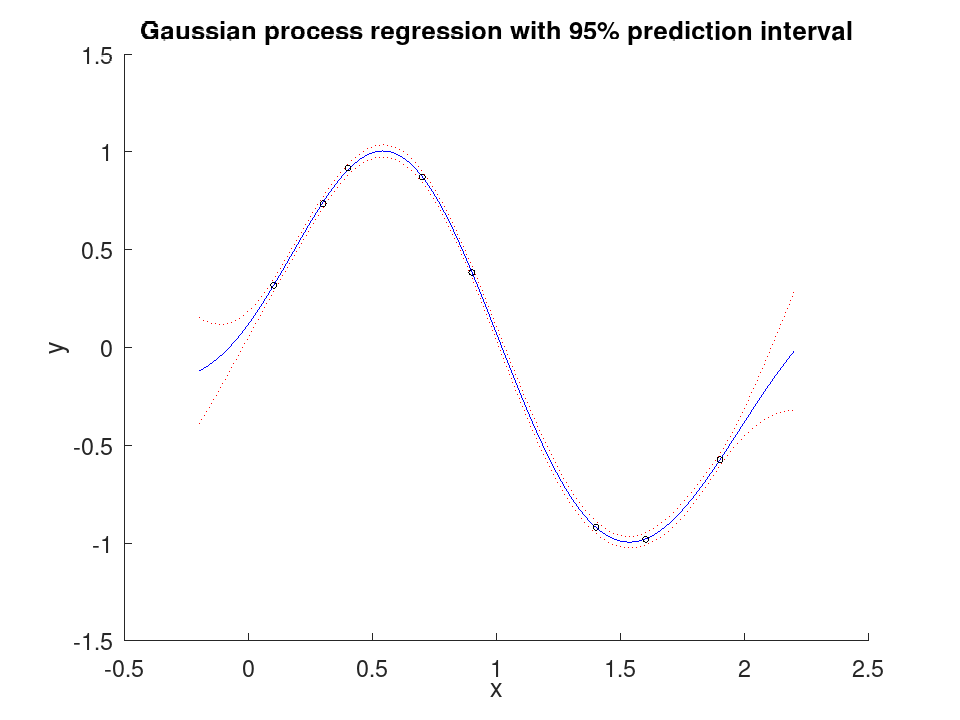
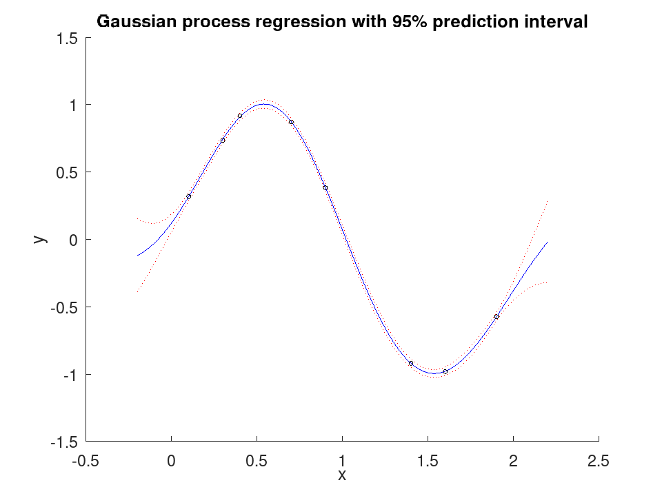
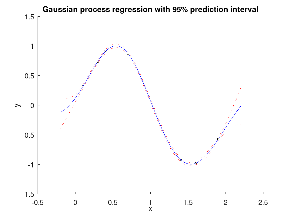
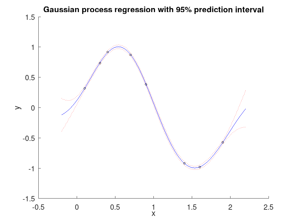
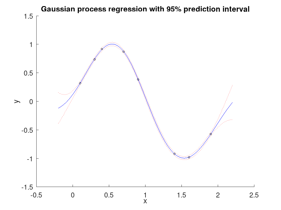
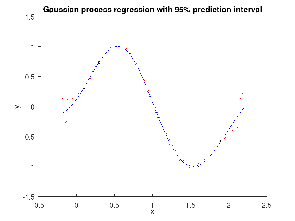
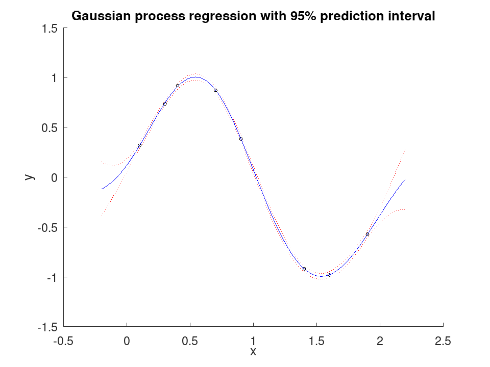
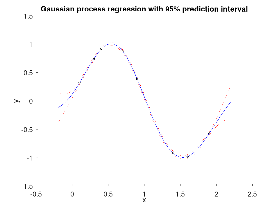
Fit a Gaussian process to noisy observations of a smooth function and show the prediction interval widening away from the data.
 x = [0.1; 0.3; 0.4; 0.7; 0.9; 1.4; 1.6; 1.9]';
 x = x(:);
 y = sin (3 * x) + 0.05 * cos (11 * x);
 Mdl = fitrgp (x, y);
 xq = linspace (-0.2, 2.2, 200)';
 [yq, ~, yint] = predict (Mdl, xq);
 figure ('visible', 'off');
 hold on;
 plot (xq, yint(:,1), 'r:');
 plot (xq, yint(:,2), 'r:');
 plot (xq, yq, 'b-');
 plot (x, y, 'ko');
 hold off;
 xlabel ('x');
 ylabel ('y');
 title ('Gaussian process regression with 95% prediction interval');
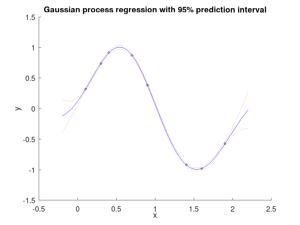
An Nx1 numeric vector, as it was supplied to the constructor. This property is read-only.
Fit a Gaussian process to noisy observations of a smooth function and show the prediction interval widening away from the data.
 x = [0.1; 0.3; 0.4; 0.7; 0.9; 1.4; 1.6; 1.9]';
 x = x(:);
 y = sin (3 * x) + 0.05 * cos (11 * x);
 Mdl = fitrgp (x, y);
 xq = linspace (-0.2, 2.2, 200)';
 [yq, ~, yint] = predict (Mdl, xq);
 figure ('visible', 'off');
 hold on;
 plot (xq, yint(:,1), 'r:');
 plot (xq, yint(:,2), 'r:');
 plot (xq, yq, 'b-');
 plot (x, y, 'ko');
 hold off;
 xlabel ('x');
 ylabel ('y');
 title ('Gaussian process regression with 95% prediction interval');
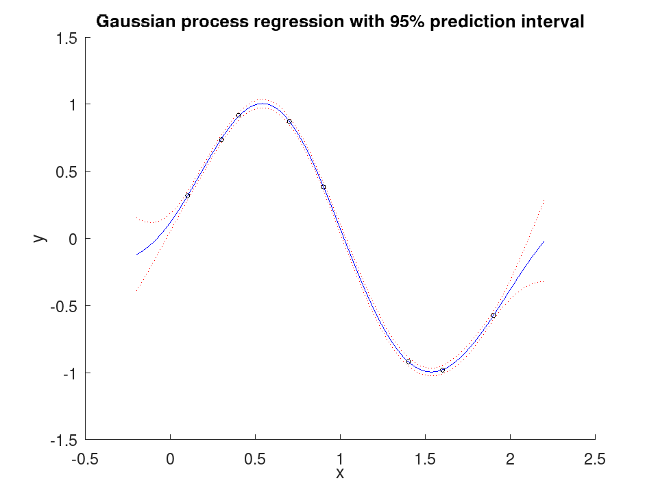
A positive integer scalar, counting the rows whose response is not missing. A row missing a predictor is counted, as in MATLAB, though the fit leaves it out. This property is read-only.
Fit a Gaussian process to noisy observations of a smooth function and show the prediction interval widening away from the data.
 x = [0.1; 0.3; 0.4; 0.7; 0.9; 1.4; 1.6; 1.9]';
 x = x(:);
 y = sin (3 * x) + 0.05 * cos (11 * x);
 Mdl = fitrgp (x, y);
 xq = linspace (-0.2, 2.2, 200)';
 [yq, ~, yint] = predict (Mdl, xq);
 figure ('visible', 'off');
 hold on;
 plot (xq, yint(:,1), 'r:');
 plot (xq, yint(:,2), 'r:');
 plot (xq, yq, 'b-');
 plot (x, y, 'ko');
 hold off;
 xlabel ('x');
 ylabel ('y');
 title ('Gaussian process regression with 95% prediction interval');
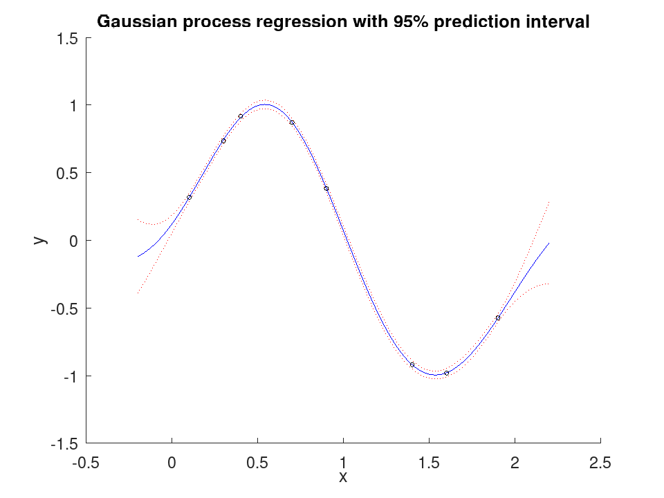
A logical vector with one element per row of the data as supplied, true where the row was used, false where its response was missing. It is empty when no row was dropped. This property is read-only.
Fit a Gaussian process to noisy observations of a smooth function and show the prediction interval widening away from the data.
 x = [0.1; 0.3; 0.4; 0.7; 0.9; 1.4; 1.6; 1.9]';
 x = x(:);
 y = sin (3 * x) + 0.05 * cos (11 * x);
 Mdl = fitrgp (x, y);
 xq = linspace (-0.2, 2.2, 200)';
 [yq, ~, yint] = predict (Mdl, xq);
 figure ('visible', 'off');
 hold on;
 plot (xq, yint(:,1), 'r:');
 plot (xq, yint(:,2), 'r:');
 plot (xq, yq, 'b-');
 plot (x, y, 'ko');
 hold off;
 xlabel ('x');
 ylabel ('y');
 title ('Gaussian process regression with 95% prediction interval');
An Nx1 vector, one weight per observation used to train the
model, scaled to sum to one and of the class of the 'Weights'
given, single or double. This property is read-only.
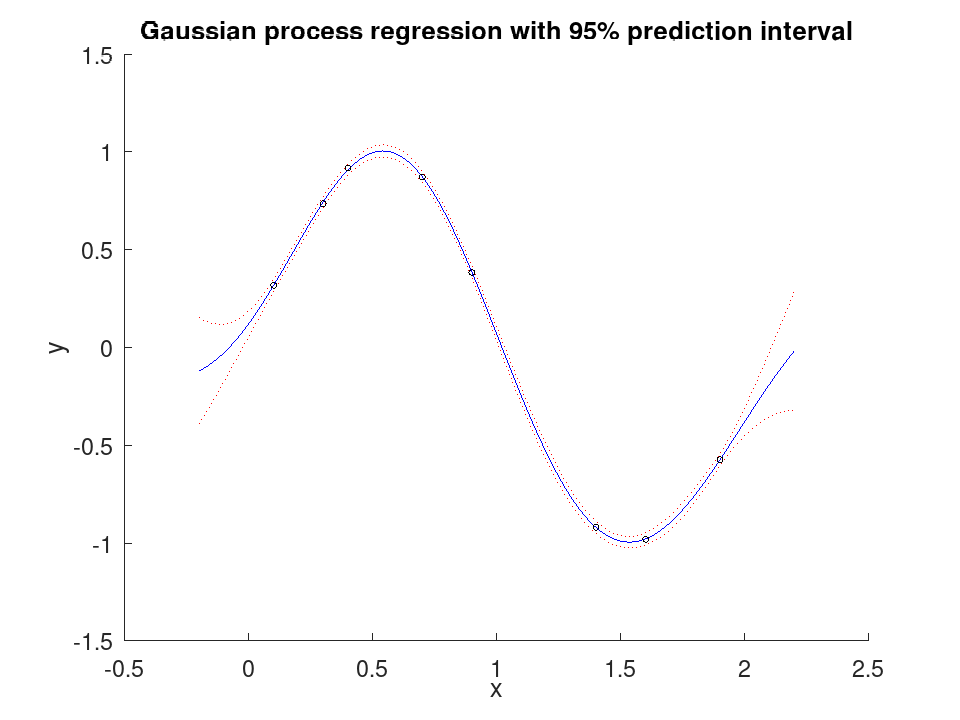
Fit a Gaussian process to noisy observations of a smooth function and show the prediction interval widening away from the data.
 x = [0.1; 0.3; 0.4; 0.7; 0.9; 1.4; 1.6; 1.9]';
 x = x(:);
 y = sin (3 * x) + 0.05 * cos (11 * x);
 Mdl = fitrgp (x, y);
 xq = linspace (-0.2, 2.2, 200)';
 [yq, ~, yint] = predict (Mdl, xq);
 figure ('visible', 'off');
 hold on;
 plot (xq, yint(:,1), 'r:');
 plot (xq, yint(:,2), 'r:');
 plot (xq, yq, 'b-');
 plot (x, y, 'ko');
 hold off;
 xlabel ('x');
 ylabel ('y');
 title ('Gaussian process regression with 95% prediction interval');
A cell array of character vectors, one per column of X. This
property is read-only.
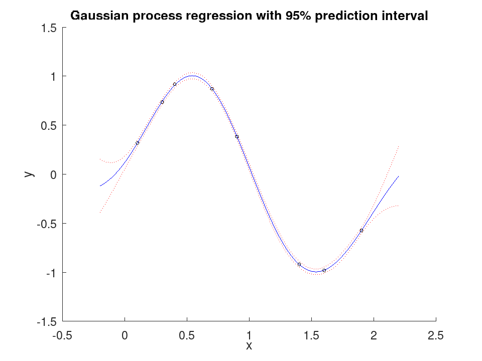
Fit a Gaussian process to noisy observations of a smooth function and show the prediction interval widening away from the data.
 x = [0.1; 0.3; 0.4; 0.7; 0.9; 1.4; 1.6; 1.9]';
 x = x(:);
 y = sin (3 * x) + 0.05 * cos (11 * x);
 Mdl = fitrgp (x, y);
 xq = linspace (-0.2, 2.2, 200)';
 [yq, ~, yint] = predict (Mdl, xq);
 figure ('visible', 'off');
 hold on;
 plot (xq, yint(:,1), 'r:');
 plot (xq, yint(:,2), 'r:');
 plot (xq, yq, 'b-');
 plot (x, y, 'ko');
 hold off;
 xlabel ('x');
 ylabel ('y');
 title ('Gaussian process regression with 95% prediction interval');
A cell array of character vectors. It differs from
PredictorNames only where a categorical predictor has been
expanded into indicator variables. This property is read-only.
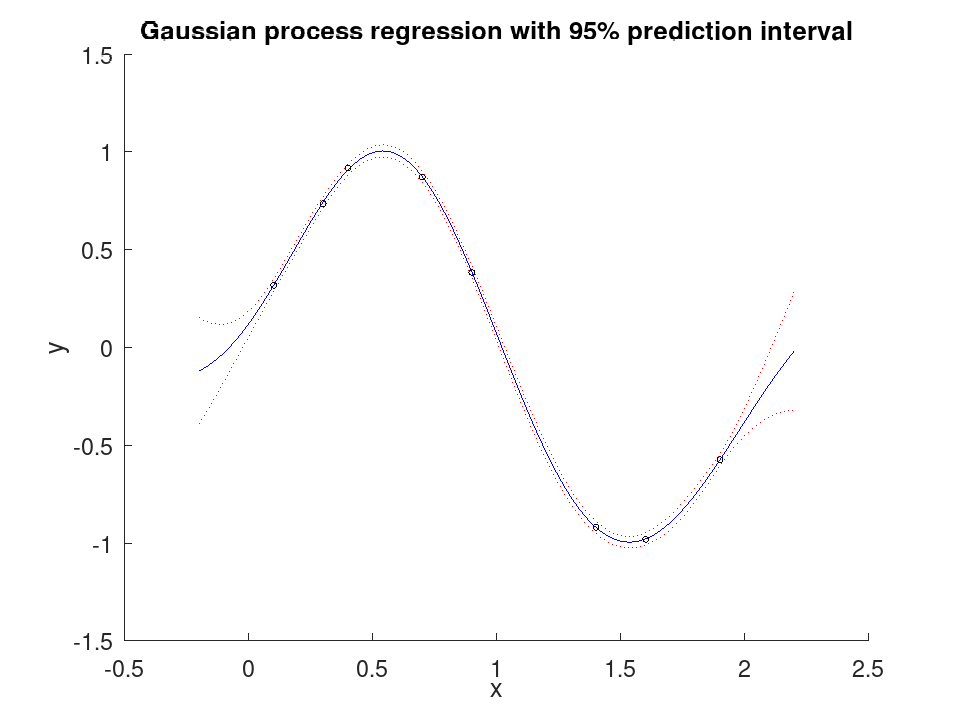
Fit a Gaussian process to noisy observations of a smooth function and show the prediction interval widening away from the data.
 x = [0.1; 0.3; 0.4; 0.7; 0.9; 1.4; 1.6; 1.9]';
 x = x(:);
 y = sin (3 * x) + 0.05 * cos (11 * x);
 Mdl = fitrgp (x, y);
 xq = linspace (-0.2, 2.2, 200)';
 [yq, ~, yint] = predict (Mdl, xq);
 figure ('visible', 'off');
 hold on;
 plot (xq, yint(:,1), 'r:');
 plot (xq, yint(:,2), 'r:');
 plot (xq, yq, 'b-');
 plot (x, y, 'ko');
 hold off;
 xlabel ('x');
 ylabel ('y');
 title ('Gaussian process regression with 95% prediction interval');
A character vector. This property is read-only.
Fit a Gaussian process to noisy observations of a smooth function and show the prediction interval widening away from the data.
 x = [0.1; 0.3; 0.4; 0.7; 0.9; 1.4; 1.6; 1.9]';
 x = x(:);
 y = sin (3 * x) + 0.05 * cos (11 * x);
 Mdl = fitrgp (x, y);
 xq = linspace (-0.2, 2.2, 200)';
 [yq, ~, yint] = predict (Mdl, xq);
 figure ('visible', 'off');
 hold on;
 plot (xq, yint(:,1), 'r:');
 plot (xq, yint(:,2), 'r:');
 plot (xq, yq, 'b-');
 plot (x, y, 'ko');
 hold off;
 xlabel ('x');
 ylabel ('y');
 title ('Gaussian process regression with 95% prediction interval');
A vector of positive integers indexing the columns of X that
hold categorical predictors, or empty when none does. This property is
read-only.
Fit a Gaussian process to noisy observations of a smooth function and show the prediction interval widening away from the data.
 x = [0.1; 0.3; 0.4; 0.7; 0.9; 1.4; 1.6; 1.9]';
 x = x(:);
 y = sin (3 * x) + 0.05 * cos (11 * x);
 Mdl = fitrgp (x, y);
 xq = linspace (-0.2, 2.2, 200)';
 [yq, ~, yint] = predict (Mdl, xq);
 figure ('visible', 'off');
 hold on;
 plot (xq, yint(:,1), 'r:');
 plot (xq, yint(:,2), 'r:');
 plot (xq, yq, 'b-');
 plot (x, y, 'ko');
 hold off;
 xlabel ('x');
 ylabel ('y');
 title ('Gaussian process regression with 95% prediction interval');
A cell array with one entry per predictor, holding that predictor’s bin edges where the model discretized it before fitting. It is empty here and stays empty: a Gaussian process takes its predictors as they are.
This property is read-only.
Fit a Gaussian process to noisy observations of a smooth function and show the prediction interval widening away from the data.
 x = [0.1; 0.3; 0.4; 0.7; 0.9; 1.4; 1.6; 1.9]';
 x = x(:);
 y = sin (3 * x) + 0.05 * cos (11 * x);
 Mdl = fitrgp (x, y);
 xq = linspace (-0.2, 2.2, 200)';
 [yq, ~, yint] = predict (Mdl, xq);
 figure ('visible', 'off');
 hold on;
 plot (xq, yint(:,1), 'r:');
 plot (xq, yint(:,2), 'r:');
 plot (xq, yq, 'b-');
 plot (x, y, 'ko');
 hold off;
 xlabel ('x');
 ylabel ('y');
 title ('Gaussian process regression with 95% prediction interval');
'Exact' when the covariance parameters and the noise were
estimated by maximizing the log marginal likelihood, and 'None'
when they were kept at their initial values. This property is
read-only.
Fit a Gaussian process to noisy observations of a smooth function and show the prediction interval widening away from the data.
 x = [0.1; 0.3; 0.4; 0.7; 0.9; 1.4; 1.6; 1.9]';
 x = x(:);
 y = sin (3 * x) + 0.05 * cos (11 * x);
 Mdl = fitrgp (x, y);
 xq = linspace (-0.2, 2.2, 200)';
 [yq, ~, yint] = predict (Mdl, xq);
 figure ('visible', 'off');
 hold on;
 plot (xq, yint(:,1), 'r:');
 plot (xq, yint(:,2), 'r:');
 plot (xq, yq, 'b-');
 plot (x, y, 'ko');
 hold off;
 xlabel ('x');
 ylabel ('y');
 title ('Gaussian process regression with 95% prediction interval');
'None', 'Constant', 'Linear',
'PureQuadratic', or the function handle that was supplied. This
property is read-only.
Fit a Gaussian process to noisy observations of a smooth function and show the prediction interval widening away from the data.
 x = [0.1; 0.3; 0.4; 0.7; 0.9; 1.4; 1.6; 1.9]';
 x = x(:);
 y = sin (3 * x) + 0.05 * cos (11 * x);
 Mdl = fitrgp (x, y);
 xq = linspace (-0.2, 2.2, 200)';
 [yq, ~, yint] = predict (Mdl, xq);
 figure ('visible', 'off');
 hold on;
 plot (xq, yint(:,1), 'r:');
 plot (xq, yint(:,2), 'r:');
 plot (xq, yq, 'b-');
 plot (x, y, 'ko');
 hold off;
 xlabel ('x');
 ylabel ('y');
 title ('Gaussian process regression with 95% prediction interval');
A numeric vector with one element per basis term, empty when the basis
is 'None'. This property is read-only.
Fit a Gaussian process to noisy observations of a smooth function and show the prediction interval widening away from the data.
 x = [0.1; 0.3; 0.4; 0.7; 0.9; 1.4; 1.6; 1.9]';
 x = x(:);
 y = sin (3 * x) + 0.05 * cos (11 * x);
 Mdl = fitrgp (x, y);
 xq = linspace (-0.2, 2.2, 200)';
 [yq, ~, yint] = predict (Mdl, xq);
 figure ('visible', 'off');
 hold on;
 plot (xq, yint(:,1), 'r:');
 plot (xq, yint(:,2), 'r:');
 plot (xq, yq, 'b-');
 plot (x, y, 'ko');
 hold off;
 xlabel ('x');
 ylabel ('y');
 title ('Gaussian process regression with 95% prediction interval');
A positive scalar. This property is read-only.
Fit a Gaussian process to noisy observations of a smooth function and show the prediction interval widening away from the data.
 x = [0.1; 0.3; 0.4; 0.7; 0.9; 1.4; 1.6; 1.9]';
 x = x(:);
 y = sin (3 * x) + 0.05 * cos (11 * x);
 Mdl = fitrgp (x, y);
 xq = linspace (-0.2, 2.2, 200)';
 [yq, ~, yint] = predict (Mdl, xq);
 figure ('visible', 'off');
 hold on;
 plot (xq, yint(:,1), 'r:');
 plot (xq, yint(:,2), 'r:');
 plot (xq, yq, 'b-');
 plot (x, y, 'ko');
 hold off;
 xlabel ('x');
 ylabel ('y');
 title ('Gaussian process regression with 95% prediction interval');
A scalar, or empty when FitMethod is 'None' and nothing
was maximized. This property is read-only.
Fit a Gaussian process to noisy observations of a smooth function and show the prediction interval widening away from the data.
 x = [0.1; 0.3; 0.4; 0.7; 0.9; 1.4; 1.6; 1.9]';
 x = x(:);
 y = sin (3 * x) + 0.05 * cos (11 * x);
 Mdl = fitrgp (x, y);
 xq = linspace (-0.2, 2.2, 200)';
 [yq, ~, yint] = predict (Mdl, xq);
 figure ('visible', 'off');
 hold on;
 plot (xq, yint(:,1), 'r:');
 plot (xq, yint(:,2), 'r:');
 plot (xq, yq, 'b-');
 plot (x, y, 'ko');
 hold off;
 xlabel ('x');
 ylabel ('y');
 title ('Gaussian process regression with 95% prediction interval');
A structure holding the options the fit was performed under. MATLAB returns an object of its own class here; a structure carries the same information and is what every other learner in this package returns.
Beta, Sigma and KernelParameters are the
starting values the fit was given, empty or zero where it was
given none, as they are in MATLAB. What the fit found is reported by
the Beta and Sigma properties and by
KernelInformation. Beta defaults to a zero for every
column the basis contributes, so a 'linear' basis over three
predictors starts at four zeros.
SigmaLowerBound is the exception and is reported as it was
resolved. MATLAB publishes no top-level field of that name, keeping
it inside an Options structure this class does not carry.
The fields MATLAB reports for its approximate fitting methods
(ActiveSet, Options, OptimizerOptions,
ConstantKernelParameters, InitialStepSize,
InitialSigmaLowerBoundTolerance, Verbose and
CacheSize) are absent, this class implementing exact fitting
alone. This property is read-only.
Fit a Gaussian process to noisy observations of a smooth function and show the prediction interval widening away from the data.
 x = [0.1; 0.3; 0.4; 0.7; 0.9; 1.4; 1.6; 1.9]';
 x = x(:);
 y = sin (3 * x) + 0.05 * cos (11 * x);
 Mdl = fitrgp (x, y);
 xq = linspace (-0.2, 2.2, 200)';
 [yq, ~, yint] = predict (Mdl, xq);
 figure ('visible', 'off');
 hold on;
 plot (xq, yint(:,1), 'r:');
 plot (xq, yint(:,2), 'r:');
 plot (xq, yq, 'b-');
 plot (x, y, 'ko');
 hold off;
 xlabel ('x');
 ylabel ('y');
 title ('Gaussian process regression with 95% prediction interval');
A character vector naming the covariance function, or the function handle that was supplied. This property is read-only.
Fit a Gaussian process to noisy observations of a smooth function and show the prediction interval widening away from the data.
 x = [0.1; 0.3; 0.4; 0.7; 0.9; 1.4; 1.6; 1.9]';
 x = x(:);
 y = sin (3 * x) + 0.05 * cos (11 * x);
 Mdl = fitrgp (x, y);
 xq = linspace (-0.2, 2.2, 200)';
 [yq, ~, yint] = predict (Mdl, xq);
 figure ('visible', 'off');
 hold on;
 plot (xq, yint(:,1), 'r:');
 plot (xq, yint(:,2), 'r:');
 plot (xq, yq, 'b-');
 plot (x, y, 'ko');
 hold off;
 xlabel ('x');
 ylabel ('y');
 title ('Gaussian process regression with 95% prediction interval');
A structure with fields Name, KernelParameters and
KernelParameterNames, the last naming each parameter in the
order they are stored. This property is read-only.
Fit a Gaussian process to noisy observations of a smooth function and show the prediction interval widening away from the data.
 x = [0.1; 0.3; 0.4; 0.7; 0.9; 1.4; 1.6; 1.9]';
 x = x(:);
 y = sin (3 * x) + 0.05 * cos (11 * x);
 Mdl = fitrgp (x, y);
 xq = linspace (-0.2, 2.2, 200)';
 [yq, ~, yint] = predict (Mdl, xq);
 figure ('visible', 'off');
 hold on;
 plot (xq, yint(:,1), 'r:');
 plot (xq, yint(:,2), 'r:');
 plot (xq, yq, 'b-');
 plot (x, y, 'ko');
 hold off;
 xlabel ('x');
 ylabel ('y');
 title ('Gaussian process regression with 95% prediction interval');
'Exact'. This property is read-only.
Fit a Gaussian process to noisy observations of a smooth function and show the prediction interval widening away from the data.
 x = [0.1; 0.3; 0.4; 0.7; 0.9; 1.4; 1.6; 1.9]';
 x = x(:);
 y = sin (3 * x) + 0.05 * cos (11 * x);
 Mdl = fitrgp (x, y);
 xq = linspace (-0.2, 2.2, 200)';
 [yq, ~, yint] = predict (Mdl, xq);
 figure ('visible', 'off');
 hold on;
 plot (xq, yint(:,1), 'r:');
 plot (xq, yint(:,2), 'r:');
 plot (xq, yq, 'b-');
 plot (x, y, 'ko');
 hold off;
 xlabel ('x');
 ylabel ('y');
 title ('Gaussian process regression with 95% prediction interval');
An Nx1 numeric vector. A prediction is the basis term plus the covariance between the new point and the active set, weighted by these. This property is read-only.
Fit a Gaussian process to noisy observations of a smooth function and show the prediction interval widening away from the data.
 x = [0.1; 0.3; 0.4; 0.7; 0.9; 1.4; 1.6; 1.9]';
 x = x(:);
 y = sin (3 * x) + 0.05 * cos (11 * x);
 Mdl = fitrgp (x, y);
 xq = linspace (-0.2, 2.2, 200)';
 [yq, ~, yint] = predict (Mdl, xq);
 figure ('visible', 'off');
 hold on;
 plot (xq, yint(:,1), 'r:');
 plot (xq, yint(:,2), 'r:');
 plot (xq, yq, 'b-');
 plot (x, y, 'ko');
 hold off;
 xlabel ('x');
 ylabel ('y');
 title ('Gaussian process regression with 95% prediction interval');
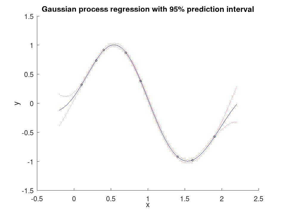
An MxP numeric matrix, standardized where the model standardized its predictors. It is the whole of the training data, since only the exact method is implemented. This property is read-only.
Fit a Gaussian process to noisy observations of a smooth function and show the prediction interval widening away from the data.
 x = [0.1; 0.3; 0.4; 0.7; 0.9; 1.4; 1.6; 1.9]';
 x = x(:);
 y = sin (3 * x) + 0.05 * cos (11 * x);
 Mdl = fitrgp (x, y);
 xq = linspace (-0.2, 2.2, 200)';
 [yq, ~, yint] = predict (Mdl, xq);
 figure ('visible', 'off');
 hold on;
 plot (xq, yint(:,1), 'r:');
 plot (xq, yint(:,2), 'r:');
 plot (xq, yq, 'b-');
 plot (x, y, 'ko');
 hold off;
 xlabel ('x');
 ylabel ('y');
 title ('Gaussian process regression with 95% prediction interval');
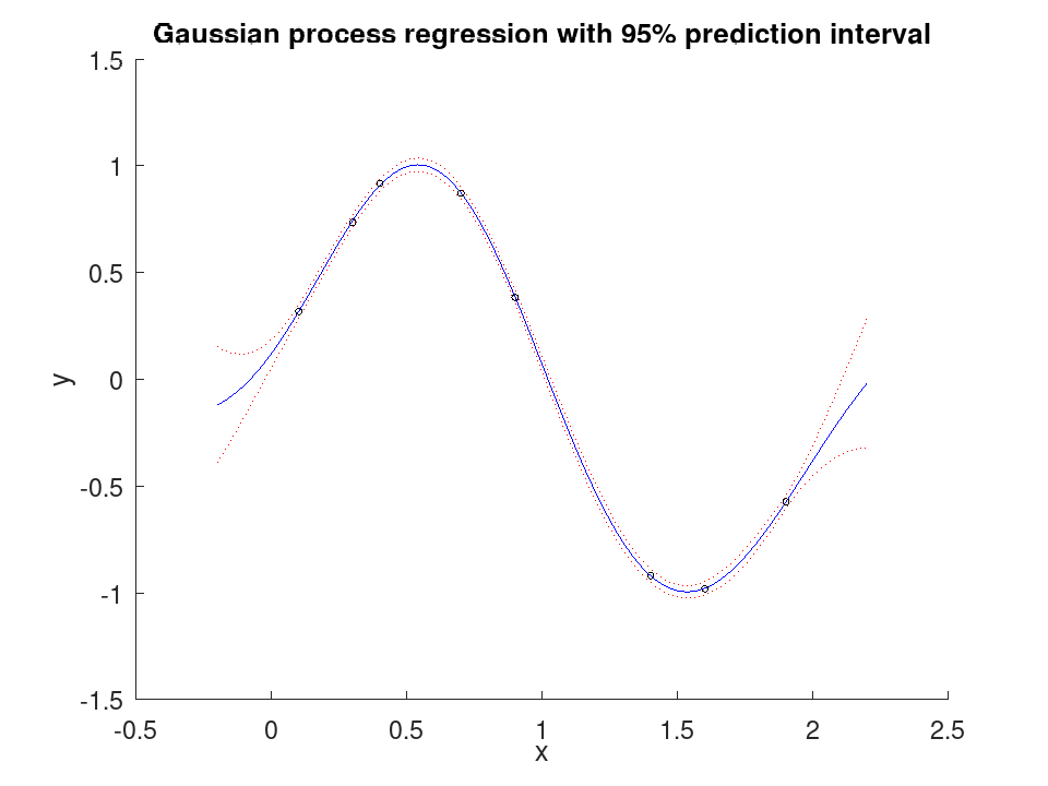
'Random'. This property is read-only.
Fit a Gaussian process to noisy observations of a smooth function and show the prediction interval widening away from the data.
 x = [0.1; 0.3; 0.4; 0.7; 0.9; 1.4; 1.6; 1.9]';
 x = x(:);
 y = sin (3 * x) + 0.05 * cos (11 * x);
 Mdl = fitrgp (x, y);
 xq = linspace (-0.2, 2.2, 200)';
 [yq, ~, yint] = predict (Mdl, xq);
 figure ('visible', 'off');
 hold on;
 plot (xq, yint(:,1), 'r:');
 plot (xq, yint(:,2), 'r:');
 plot (xq, yq, 'b-');
 plot (x, y, 'ko');
 hold off;
 xlabel ('x');
 ylabel ('y');
 title ('Gaussian process regression with 95% prediction interval');
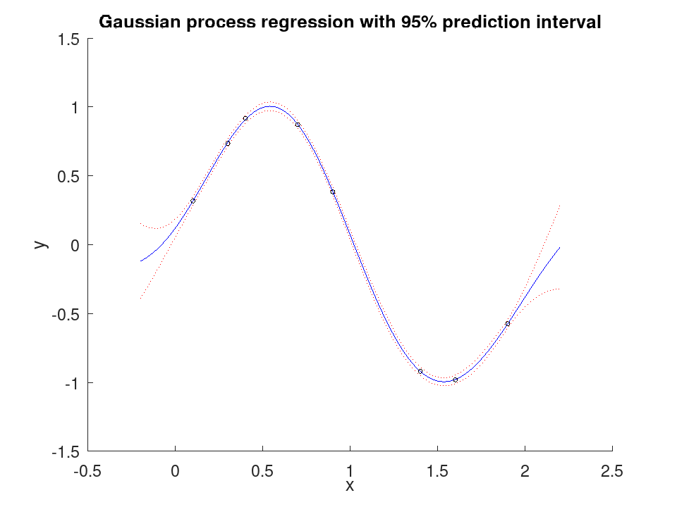
A positive integer scalar. This property is read-only.
Fit a Gaussian process to noisy observations of a smooth function and show the prediction interval widening away from the data.
 x = [0.1; 0.3; 0.4; 0.7; 0.9; 1.4; 1.6; 1.9]';
 x = x(:);
 y = sin (3 * x) + 0.05 * cos (11 * x);
 Mdl = fitrgp (x, y);
 xq = linspace (-0.2, 2.2, 200)';
 [yq, ~, yint] = predict (Mdl, xq);
 figure ('visible', 'off');
 hold on;
 plot (xq, yint(:,1), 'r:');
 plot (xq, yint(:,2), 'r:');
 plot (xq, yq, 'b-');
 plot (x, y, 'ko');
 hold off;
 xlabel ('x');
 ylabel ('y');
 title ('Gaussian process regression with 95% prediction interval');
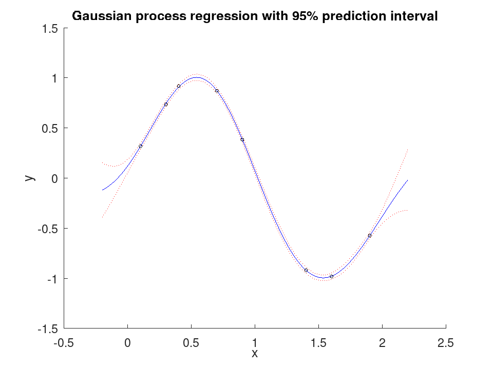
A logical vector with one element per training observation. This property is read-only.
Fit a Gaussian process to noisy observations of a smooth function and show the prediction interval widening away from the data.
 x = [0.1; 0.3; 0.4; 0.7; 0.9; 1.4; 1.6; 1.9]';
 x = x(:);
 y = sin (3 * x) + 0.05 * cos (11 * x);
 Mdl = fitrgp (x, y);
 xq = linspace (-0.2, 2.2, 200)';
 [yq, ~, yint] = predict (Mdl, xq);
 figure ('visible', 'off');
 hold on;
 plot (xq, yint(:,1), 'r:');
 plot (xq, yint(:,2), 'r:');
 plot (xq, yq, 'b-');
 plot (x, y, 'ko');
 hold off;
 xlabel ('x');
 ylabel ('y');
 title ('Gaussian process regression with 95% prediction interval');
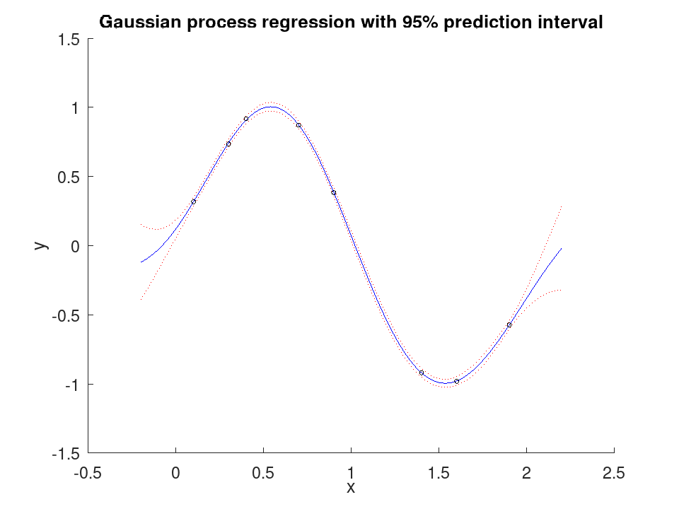
Always empty. It is declared for MATLAB compatibility, where it records the active set chosen at each iteration by a fit method that builds one. This class implements the exact method alone, which uses the whole of the training data and selects nothing, so there is no history to record. This property is read-only.
Fit a Gaussian process to noisy observations of a smooth function and show the prediction interval widening away from the data.
 x = [0.1; 0.3; 0.4; 0.7; 0.9; 1.4; 1.6; 1.9]';
 x = x(:);
 y = sin (3 * x) + 0.05 * cos (11 * x);
 Mdl = fitrgp (x, y);
 xq = linspace (-0.2, 2.2, 200)';
 [yq, ~, yint] = predict (Mdl, xq);
 figure ('visible', 'off');
 hold on;
 plot (xq, yint(:,1), 'r:');
 plot (xq, yint(:,2), 'r:');
 plot (xq, yq, 'b-');
 plot (x, y, 'ko');
 hold off;
 xlabel ('x');
 ylabel ('y');
 title ('Gaussian process regression with 95% prediction interval');
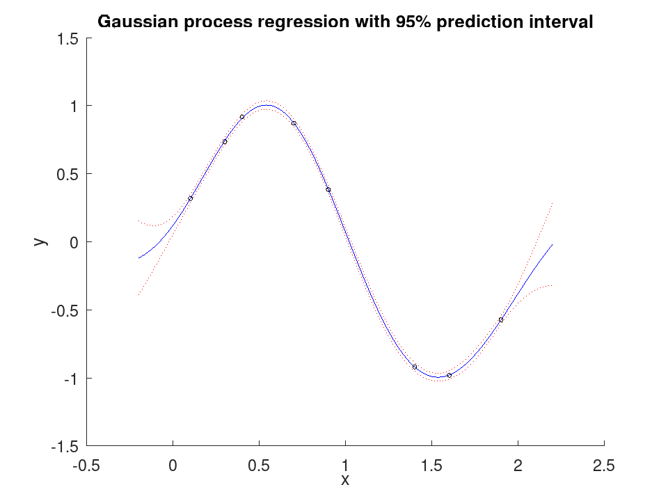
Always empty. It is declared for MATLAB compatibility, where it records a block coordinate descent. This class does not use that method, so there is nothing to report. This property is read-only.
Fit a Gaussian process to noisy observations of a smooth function and show the prediction interval widening away from the data.
 x = [0.1; 0.3; 0.4; 0.7; 0.9; 1.4; 1.6; 1.9]';
 x = x(:);
 y = sin (3 * x) + 0.05 * cos (11 * x);
 Mdl = fitrgp (x, y);
 xq = linspace (-0.2, 2.2, 200)';
 [yq, ~, yint] = predict (Mdl, xq);
 figure ('visible', 'off');
 hold on;
 plot (xq, yint(:,1), 'r:');
 plot (xq, yint(:,2), 'r:');
 plot (xq, yq, 'b-');
 plot (x, y, 'ko');
 hold off;
 xlabel ('x');
 ylabel ('y');
 title ('Gaussian process regression with 95% prediction interval');
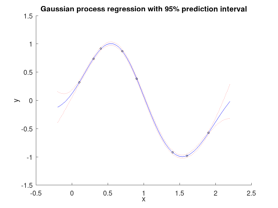
A 1xP numeric vector when the model standardized its predictors, and empty when it did not. This property is read-only.
Fit a Gaussian process to noisy observations of a smooth function and show the prediction interval widening away from the data.
 x = [0.1; 0.3; 0.4; 0.7; 0.9; 1.4; 1.6; 1.9]';
 x = x(:);
 y = sin (3 * x) + 0.05 * cos (11 * x);
 Mdl = fitrgp (x, y);
 xq = linspace (-0.2, 2.2, 200)';
 [yq, ~, yint] = predict (Mdl, xq);
 figure ('visible', 'off');
 hold on;
 plot (xq, yint(:,1), 'r:');
 plot (xq, yint(:,2), 'r:');
 plot (xq, yq, 'b-');
 plot (x, y, 'ko');
 hold off;
 xlabel ('x');
 ylabel ('y');
 title ('Gaussian process regression with 95% prediction interval');
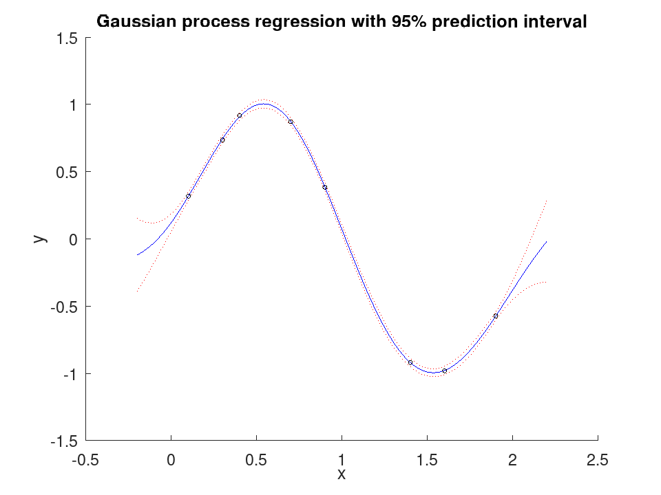
A 1xP numeric vector when the model standardized its predictors, and empty when it did not. This property is read-only.
Fit a Gaussian process to noisy observations of a smooth function and show the prediction interval widening away from the data.
 x = [0.1; 0.3; 0.4; 0.7; 0.9; 1.4; 1.6; 1.9]';
 x = x(:);
 y = sin (3 * x) + 0.05 * cos (11 * x);
 Mdl = fitrgp (x, y);
 xq = linspace (-0.2, 2.2, 200)';
 [yq, ~, yint] = predict (Mdl, xq);
 figure ('visible', 'off');
 hold on;
 plot (xq, yint(:,1), 'r:');
 plot (xq, yint(:,2), 'r:');
 plot (xq, yq, 'b-');
 plot (x, y, 'ko');
 hold off;
 xlabel ('x');
 ylabel ('y');
 title ('Gaussian process regression with 95% prediction interval');
Always empty. It is declared for MATLAB compatibility, where it holds what an automatic search over the hyperparameters found. This class fits the parameters it is given and runs no such search, so there is nothing to report. This property is read-only.
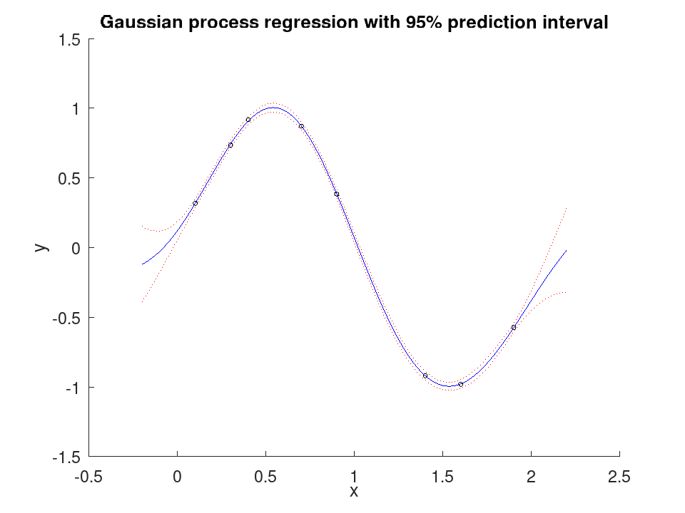
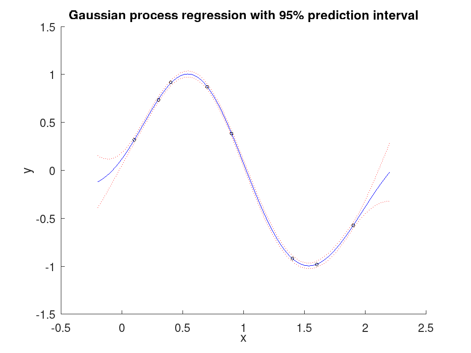
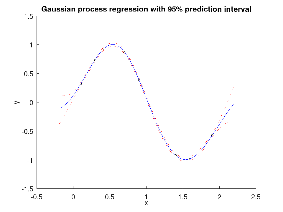
Fit a Gaussian process to noisy observations of a smooth function and show the prediction interval widening away from the data.
 x = [0.1; 0.3; 0.4; 0.7; 0.9; 1.4; 1.6; 1.9]';
 x = x(:);
 y = sin (3 * x) + 0.05 * cos (11 * x);
 Mdl = fitrgp (x, y);
 xq = linspace (-0.2, 2.2, 200)';
 [yq, ~, yint] = predict (Mdl, xq);
 figure ('visible', 'off');
 hold on;
 plot (xq, yint(:,1), 'r:');
 plot (xq, yint(:,2), 'r:');
 plot (xq, yq, 'b-');
 plot (x, y, 'ko');
 hold off;
 xlabel ('x');
 ylabel ('y');
 title ('Gaussian process regression with 95% prediction interval');
A character vector, or the text of the function handle that was supplied. Assigning to it accepts either.
Fit a Gaussian process to noisy observations of a smooth function and show the prediction interval widening away from the data.
 x = [0.1; 0.3; 0.4; 0.7; 0.9; 1.4; 1.6; 1.9]';
 x = x(:);
 y = sin (3 * x) + 0.05 * cos (11 * x);
 Mdl = fitrgp (x, y);
 xq = linspace (-0.2, 2.2, 200)';
 [yq, ~, yint] = predict (Mdl, xq);
 figure ('visible', 'off');
 hold on;
 plot (xq, yint(:,1), 'r:');
 plot (xq, yint(:,2), 'r:');
 plot (xq, yq, 'b-');
 plot (x, y, 'ko');
 hold off;
 xlabel ('x');
 ylabel ('y');
 title ('Gaussian process regression with 95% prediction interval');
The RegressionGP class offers the following public methods:
RegressionGP: obj = RegressionGP (X, Y)
RegressionGP: obj = RegressionGP (Tbl, ResponseVarName)
RegressionGP: obj = RegressionGP (Tbl, formula)
RegressionGP: obj = RegressionGP (Tbl, Y)
RegressionGP: obj = RegressionGP (…, name, value)
obj = RegressionGP (X, Y) returns a Gaussian
process regression model, obj, with X being the predictor
data and Y the continuous response of the observations in X.
- X must be an NxP numeric matrix of predictor data, where rows correspond to observations and columns to features.
- Y must be an Nx1 numeric vector holding the response of the corresponding predictor data in X. Y must have the same number of rows as X.
A Gaussian process places a prior over functions, given by the covariance
function, and conditions it on the observations. The response is
modelled as H×Beta plus a draw from that process plus independent
noise of standard deviation Sigma, where H is the explicit
basis. The covariance parameters and Sigma are estimated by
maximizing the log marginal likelihood, and Beta follows from
them in closed form as the generalized least squares estimate.
obj = RegressionGP (…, name, value)
returns a model with additional options specified by Name-Value
pair arguments listed below.
| Name | Value |
|---|---|
'KernelFunction' | A character vector naming the
covariance function, or a function handle taking two matrices of points
and a parameter vector. The default is 'squaredexponential'.
The supported names are listed below. |
'KernelParameters' | A numeric vector of initial values for the covariance parameters. Its length depends on the covariance function. These are starting values for the optimization, not fixed values. |
'BasisFunction' | A character vector naming the explicit
basis, one of 'none', 'constant', 'linear' or
'pureQuadratic', or a function handle taking X and
returning the basis matrix. The default is 'constant'. |
'Beta' | A numeric vector of basis coefficients. These
are used as known values only when 'FitMethod' is 'none'. |
'Sigma' | A positive scalar, the initial value of the
noise standard deviation. The default is
std (Y) / sqrt (2). |
'ConstantSigma' | A logical scalar. When true
the noise standard deviation is held at its initial value instead of
being estimated. The default is false. |
'SigmaLowerBound' | A positive scalar bounding the noise
standard deviation from below. The default is
1e-2 * std (Y). |
'FitMethod' | A character vector, either 'exact'
to estimate the parameters or 'none' to keep them at their
initial values. The default is 'exact'. |
'PredictMethod' | A character vector. Only
'exact' is implemented, which is also the only method under which
a standard deviation and a prediction interval are available. |
'Optimizer' | A character vector naming the optimizer
used to maximize the log marginal likelihood. 'quasinewton' and
'fminunc' name the same dense solver and are the default,
'lbfgs' selects limited-memory BFGS, which holds a fixed number
of curvature pairs rather than a full inverse Hessian and is the cheaper
choice when the kernel carries many parameters, and 'fminsearch'
is derivative-free. |
'Standardize' | A logical scalar specifying whether the
predictor data should be centred and scaled before training. The same
transformation is applied by predict. The default is
false. |
'CategoricalPredictors' | The categorical predictors, as
indices, as a logical vector with one element per predictor, or as
'all'. Each is dummy coded in its place, one column of zeros and
ones per distinct value it takes in the training data, named as in
'x1 == 2', and the coded columns are not standardized. X
keeps the predictors as given. A row holding a value the training data
did not is predicted as a row missing a predictor, the weighted lower
median of the training response. A predictor may be named rather than
indexed, as a character matrix of one padded name per row, a string array
or a cellstr; a name must match an entry of 'PredictorNames'
exactly, its case included. |
'Weights' | An Nx1 single or double vector of
non-negative observation weights. The default is a vector of ones. The
model’s W keeps the class of the weights, while every computation
runs in double. |
'PredictorNames' | A cell array of character vectors naming the predictors, in the order they appear in X. |
'ResponseName' | A character vector naming the response.
The default is 'Y'. |
'ResponseTransform' | A character vector or a function
handle applied to the response the model predicts. The default is
'none'. |
The supported values for 'KernelFunction' are:
| Value | Parameters |
|---|---|
'exponential' | [SigmaL; SigmaF] |
'squaredexponential' | [SigmaL; SigmaF] |
'matern32' | [SigmaL; SigmaF] |
'matern52' | [SigmaL; SigmaF] |
'rationalquadratic' | [SigmaL; AlphaRQ; SigmaF] |
'ardexponential' | [LengthScale1; …; SigmaF] |
'ardsquaredexponential' | [LengthScale1; …; SigmaF] |
'ardmatern32' | [LengthScale1; …; SigmaF] |
'ardmatern52' | [LengthScale1; …; SigmaF] |
'ardrationalquadratic' | [LengthScale1; …; AlphaRQ; SigmaF] |
The automatic relevance determination kernels carry one length scale per predictor, so a predictor the response does not depend on is given a large length scale and stops contributing.
The supported values for 'ResponseTransform' are:
| Value | Description |
|---|---|
'none' | x (no transformation) |
'identity' | x (no transformation) |
'exp' | exp (x) |
'log' | log (x) |
Two deviations from MATLAB are deliberate and documented. The distance
between points is accumulated one predictor at a time instead of by the
expanded form MATLAB uses by default, because the expanded form does not
return exactly zero for a point against itself and the rough kernels
amplify that residue through their square root. The approximate fitting
and prediction methods, 'sd', 'sr', 'fic' and
'bcd', together with the active set options that serve them, are
not implemented and are refused rather than silently ignored.
See also: fitrgp, CompactRegressionGP, RegressionSVM, RegressionGAM
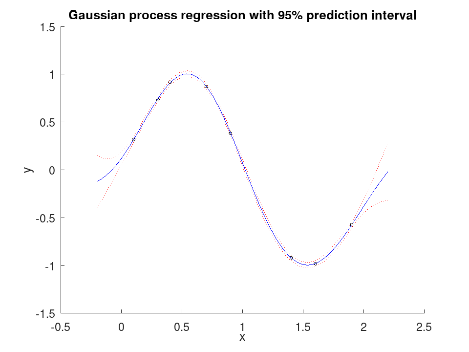
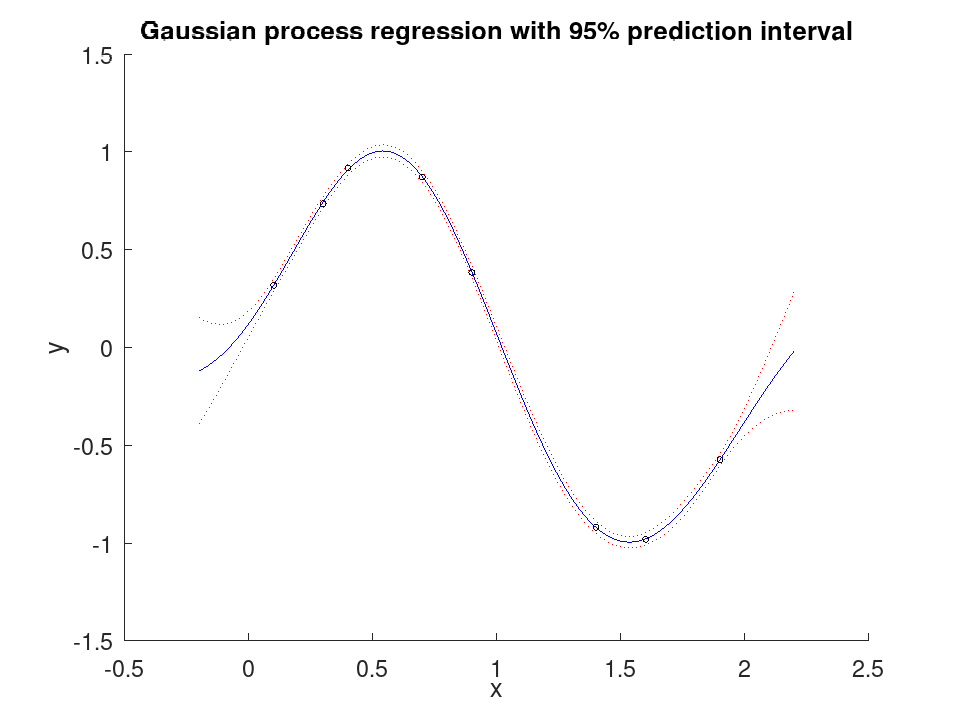
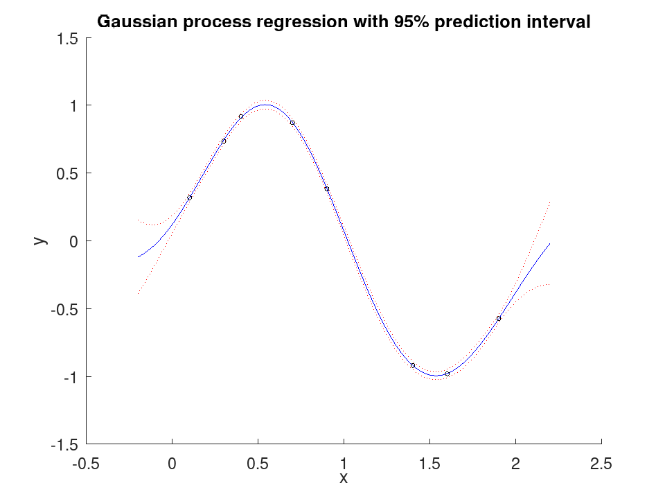
Fit a Gaussian process to noisy observations of a smooth function and show the prediction interval widening away from the data.
 x = [0.1; 0.3; 0.4; 0.7; 0.9; 1.4; 1.6; 1.9]';
 x = x(:);
 y = sin (3 * x) + 0.05 * cos (11 * x);
 Mdl = fitrgp (x, y);
 xq = linspace (-0.2, 2.2, 200)';
 [yq, ~, yint] = predict (Mdl, xq);
 figure ('visible', 'off');
 hold on;
 plot (xq, yint(:,1), 'r:');
 plot (xq, yint(:,2), 'r:');
 plot (xq, yq, 'b-');
 plot (x, y, 'ko');
 hold off;
 xlabel ('x');
 ylabel ('y');
 title ('Gaussian process regression with 95% prediction interval');
RegressionGP: yFit = predict (obj, XC)
RegressionGP: [yFit, ySD, yInt] = predict (obj, XC)
RegressionGP: […] = predict (…, 'Alpha', alpha)
yFit = predict (obj, XC) returns the predicted
response of the RegressionGP model obj at the points in
XC, which must have as many columns as the model has predictors.
[yFit, ySD, yInt] = predict (…) also
returns the standard deviation of each predicted response and the
prediction intervals. The standard deviation is that of a new
response, so it carries the noise as well as the uncertainty of
the latent function, and the interval is the normal quantile of the
level times it.
[…] = predict (…, sets
the significance level of the intervals, so that they are
100 × (1 - alpha) per cent intervals. alpha must be
a scalar in the range [0, 1] and defaults to 0.05.
'Alpha', alpha)
The new data may be a table, whose variables are matched to the predictors the model was fitted on by name and not by position: one the model was not fitted on is passed over, one it needs and cannot find is named, and a value holding a level is coded as that level was coded at fitting.
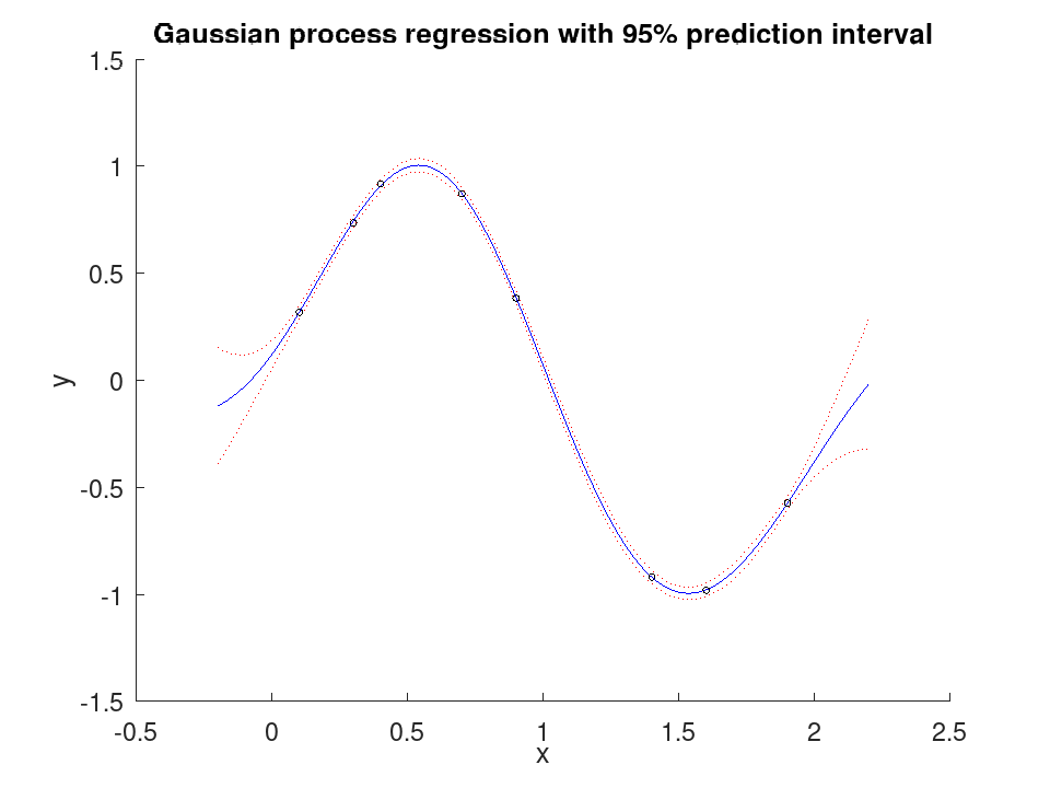
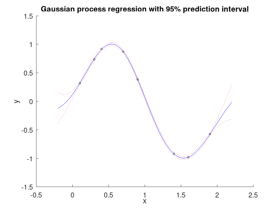
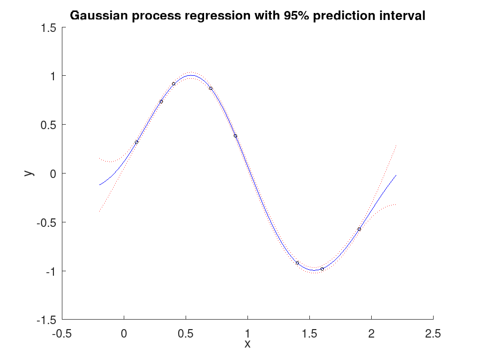
Fit a Gaussian process to noisy observations of a smooth function and show the prediction interval widening away from the data.
 x = [0.1; 0.3; 0.4; 0.7; 0.9; 1.4; 1.6; 1.9]';
 x = x(:);
 y = sin (3 * x) + 0.05 * cos (11 * x);
 Mdl = fitrgp (x, y);
 xq = linspace (-0.2, 2.2, 200)';
 [yq, ~, yint] = predict (Mdl, xq);
 figure ('visible', 'off');
 hold on;
 plot (xq, yint(:,1), 'r:');
 plot (xq, yint(:,2), 'r:');
 plot (xq, yq, 'b-');
 plot (x, y, 'ko');
 hold off;
 xlabel ('x');
 ylabel ('y');
 title ('Gaussian process regression with 95% prediction interval');
RegressionGP: yFit = resubPredict (obj)
RegressionGP: [yFit, ySD, yInt] = resubPredict (obj)
yFit = resubPredict (obj) returns the response the
RegressionGP model obj predicts at its own training data,
and the further outputs are those of predict.
Fit a Gaussian process to noisy observations of a smooth function and show the prediction interval widening away from the data.
 x = [0.1; 0.3; 0.4; 0.7; 0.9; 1.4; 1.6; 1.9]';
 x = x(:);
 y = sin (3 * x) + 0.05 * cos (11 * x);
 Mdl = fitrgp (x, y);
 xq = linspace (-0.2, 2.2, 200)';
 [yq, ~, yint] = predict (Mdl, xq);
 figure ('visible', 'off');
 hold on;
 plot (xq, yint(:,1), 'r:');
 plot (xq, yint(:,2), 'r:');
 plot (xq, yq, 'b-');
 plot (x, y, 'ko');
 hold off;
 xlabel ('x');
 ylabel ('y');
 title ('Gaussian process regression with 95% prediction interval');
RegressionGP: L = loss (obj, X, Y)
RegressionGP: L = loss (obj, Tbl, ResponseVarName)
RegressionGP: L = loss (obj, Tbl)
RegressionGP: L = loss (…, name, value)
L = loss (obj, X, Y) returns the mean
squared error of the model obj on the data X and Y.
X may also be a table Tbl, whose variables are matched to
the predictors the model was fitted on by name and not by position.
loss (obj, Tbl, ResponseVarName) takes the
response from the variable ResponseVarName names, and
loss (obj, Tbl) from the variable the model was
fitted on. The response may also be given beside the table as
Y.
L = loss (…, name, value) accepts
'LossFun', either 'mse', 'mae',
'epsiloninsensitive' or a function handle taking the observed
and the predicted response, and 'Weights', a vector of
non-negative observation weights.
Fit a Gaussian process to noisy observations of a smooth function and show the prediction interval widening away from the data.
 x = [0.1; 0.3; 0.4; 0.7; 0.9; 1.4; 1.6; 1.9]';
 x = x(:);
 y = sin (3 * x) + 0.05 * cos (11 * x);
 Mdl = fitrgp (x, y);
 xq = linspace (-0.2, 2.2, 200)';
 [yq, ~, yint] = predict (Mdl, xq);
 figure ('visible', 'off');
 hold on;
 plot (xq, yint(:,1), 'r:');
 plot (xq, yint(:,2), 'r:');
 plot (xq, yq, 'b-');
 plot (x, y, 'ko');
 hold off;
 xlabel ('x');
 ylabel ('y');
 title ('Gaussian process regression with 95% prediction interval');
RegressionGP: L = resubLoss (obj)
RegressionGP: L = resubLoss (…, name, value)
L = resubLoss (obj) returns the loss of the model
obj on the data it was trained on, and accepts the same
Name-Value pairs as loss.
Fit a Gaussian process to noisy observations of a smooth function and show the prediction interval widening away from the data.
 x = [0.1; 0.3; 0.4; 0.7; 0.9; 1.4; 1.6; 1.9]';
 x = x(:);
 y = sin (3 * x) + 0.05 * cos (11 * x);
 Mdl = fitrgp (x, y);
 xq = linspace (-0.2, 2.2, 200)';
 [yq, ~, yint] = predict (Mdl, xq);
 figure ('visible', 'off');
 hold on;
 plot (xq, yint(:,1), 'r:');
 plot (xq, yint(:,2), 'r:');
 plot (xq, yq, 'b-');
 plot (x, y, 'ko');
 hold off;
 xlabel ('x');
 ylabel ('y');
 title ('Gaussian process regression with 95% prediction interval');
RegressionGP: [loores, neff] = postFitStatistics (obj)
[loores, neff] = postFitStatistics (obj)
returns the Nx1 vector of leave-one-out residuals of the model
obj, and the number of effective parameters the fit uses. Neither
requires refitting the model: both follow from the factorization the fit
already produced.
The coefficients of the explicit basis are treated as estimated, which
is what FitMethod 'Exact' makes them, while the
covariance parameters and the noise are treated as known.
Fit a Gaussian process to noisy observations of a smooth function and show the prediction interval widening away from the data.
 x = [0.1; 0.3; 0.4; 0.7; 0.9; 1.4; 1.6; 1.9]';
 x = x(:);
 y = sin (3 * x) + 0.05 * cos (11 * x);
 Mdl = fitrgp (x, y);
 xq = linspace (-0.2, 2.2, 200)';
 [yq, ~, yint] = predict (Mdl, xq);
 figure ('visible', 'off');
 hold on;
 plot (xq, yint(:,1), 'r:');
 plot (xq, yint(:,2), 'r:');
 plot (xq, yq, 'b-');
 plot (x, y, 'ko');
 hold off;
 xlabel ('x');
 ylabel ('y');
 title ('Gaussian process regression with 95% prediction interval');
RegressionGP: CVMdl = crossval (obj)
RegressionGP: CVMdl = crossval (…, name, value)
CVMdl = crossval (obj) returns a
RegressionPartitionedModel built from the model obj by
ten-fold cross validation.
CVMdl = crossval (…, name, value) accepts
'KFold', 'Holdout', 'Leaveout' and
'CVPartition', of which at most one may be given.
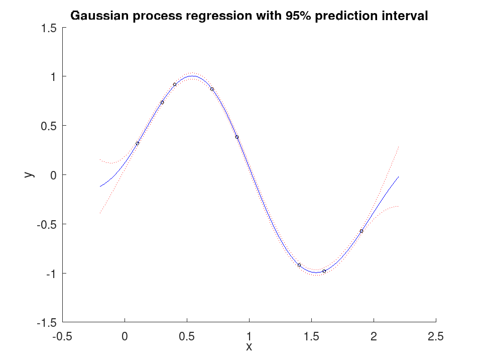
Fit a Gaussian process to noisy observations of a smooth function and show the prediction interval widening away from the data.
 x = [0.1; 0.3; 0.4; 0.7; 0.9; 1.4; 1.6; 1.9]';
 x = x(:);
 y = sin (3 * x) + 0.05 * cos (11 * x);
 Mdl = fitrgp (x, y);
 xq = linspace (-0.2, 2.2, 200)';
 [yq, ~, yint] = predict (Mdl, xq);
 figure ('visible', 'off');
 hold on;
 plot (xq, yint(:,1), 'r:');
 plot (xq, yint(:,2), 'r:');
 plot (xq, yq, 'b-');
 plot (x, y, 'ko');
 hold off;
 xlabel ('x');
 ylabel ('y');
 title ('Gaussian process regression with 95% prediction interval');
RegressionGP: CMdl = compact (obj)
CMdl = compact (obj) returns a
CompactRegressionGP object holding what is needed to predict
and nothing else: the training data, the response and everything that
describes them are dropped.
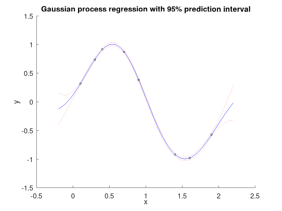
Fit a Gaussian process to noisy observations of a smooth function and show the prediction interval widening away from the data.
 x = [0.1; 0.3; 0.4; 0.7; 0.9; 1.4; 1.6; 1.9]';
 x = x(:);
 y = sin (3 * x) + 0.05 * cos (11 * x);
 Mdl = fitrgp (x, y);
 xq = linspace (-0.2, 2.2, 200)';
 [yq, ~, yint] = predict (Mdl, xq);
 figure ('visible', 'off');
 hold on;
 plot (xq, yint(:,1), 'r:');
 plot (xq, yint(:,2), 'r:');
 plot (xq, yq, 'b-');
 plot (x, y, 'ko');
 hold off;
 xlabel ('x');
 ylabel ('y');
 title ('Gaussian process regression with 95% prediction interval');
RegressionGP: savemodel (obj, filename)
savemodel (obj, filename) saves the model obj
into filename in a form loadmodel can read back.
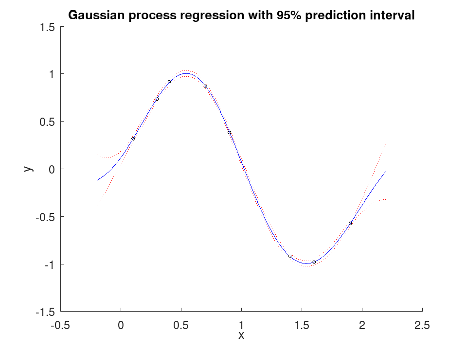
Fit a Gaussian process to noisy observations of a smooth function and show the prediction interval widening away from the data.
 x = [0.1; 0.3; 0.4; 0.7; 0.9; 1.4; 1.6; 1.9]';
 x = x(:);
 y = sin (3 * x) + 0.05 * cos (11 * x);
 Mdl = fitrgp (x, y);
 xq = linspace (-0.2, 2.2, 200)';
 [yq, ~, yint] = predict (Mdl, xq);
 figure ('visible', 'off');
 hold on;
 plot (xq, yint(:,1), 'r:');
 plot (xq, yint(:,2), 'r:');
 plot (xq, yq, 'b-');
 plot (x, y, 'ko');
 hold off;
 xlabel ('x');
 ylabel ('y');
 title ('Gaussian process regression with 95% prediction interval');
Examples
 x = [0.1; 0.3; 0.4; 0.7; 0.9; 1.4; 1.6; 1.9]';
 x = x(:);
 y = sin (3 * x) + 0.05 * cos (11 * x);
 Mdl = fitrgp (x, y);
 xq = linspace (-0.2, 2.2, 200)';
 [yq, ~, yint] = predict (Mdl, xq);
 figure ('visible', 'off');
 hold on;
 plot (xq, yint(:,1), 'r:');
 plot (xq, yint(:,2), 'r:');
 plot (xq, yq, 'b-');
 plot (x, y, 'ko');
 hold off;
 xlabel ('x');
 ylabel ('y');
 title ('Gaussian process regression with 95% prediction interval');