Categories &
Functions List
- adtest
- anova
- anova1
- anova2
- anovan
- ansaribradley
- barttest
- binotest
- chi2gof
- chi2test
- correlation_test
- detectdrift
- dwtest
- fishertest
- friedman
- hotelling_t2test
- hotelling_t2test2
- jbtest
- knntest
- kruskalwallis
- kstest
- kstest2
- lillietest
- manova1
- mcnemar_test
- meanEffectSize
- mmdtest
- multcompare
- ranksum
- regression_ftest
- regression_ttest
- runstest
- signrank
- signtest
- stats.drift.DriftDiagnostics
- swtest
- ttest
- ttest2
- vartest
- vartest2
- vartestn
- ztest
- ztest2
- CompactLinearModel
- CoxModel
- coxphfit
- fitcox
- fitglm
- fitglme
- fitlm
- fitlme
- fitlmematrix
- fitnlm
- fitrm
- GeneralizedLinearMixedModel
- GeneralizedLinearModel
- glmfit
- glmval
- invpred
- lasso
- lassoglm
- LinearFormula
- LinearMixedModel
- LinearModel
- logistic_regression
- mnrfit
- mnrval
- monotone_smooth
- mvregress
- mvregresslike
- nlinfit
- nlparci
- nlpredci
- NonLinearModel
- plsregress
- regress
- regress_gp
- RepeatedMeasuresModel
- ridge
- robustfit
- stepwisefit
- stepwiseglm
- stepwiselm
- ClassificationBaggedEnsemble
- ClassificationDiscriminant
- ClassificationECOC
- ClassificationEnsemble
- ClassificationGAM
- ClassificationKernel
- ClassificationKNN
- ClassificationLinear
- ClassificationNaiveBayes
- ClassificationNeuralNetwork
- ClassificationPartitionedECOC
- ClassificationPartitionedEnsemble
- ClassificationPartitionedKernel
- ClassificationPartitionedLinear
- ClassificationPartitionedModel
- ClassificationSVM
- ClassificationTree
- CompactClassificationDiscriminant
- CompactClassificationECOC
- CompactClassificationEnsemble
- CompactClassificationGAM
- CompactClassificationNaiveBayes
- CompactClassificationNeuralNetwork
- CompactClassificationSVM
- CompactClassificationTree
- CompactRegressionGAM
- CompactRegressionEnsemble
- CompactRegressionGP
- CompactRegressionNeuralNetwork
- CompactRegressionSVM
- CompactRegressionTree
- CompactTreeBagger
- designecoc
- fcnnpredict
- fcnntrain
- fitcdiscr
- fitcecoc
- fitcensemble
- fitcgam
- fitckernel
- fitcknn
- fitclinear
- fitcnb
- fitcnet
- fitcsvm
- fitctree
- fitrensemble
- fitrgam
- fitrgp
- fitrkernel
- fitrlinear
- fitrnet
- fitrsvm
- fitrtree
- gamboostinter
- gamboostpairs
- gamboostpredict
- gamboosttrain
- gampredict
- gamtrain
- partialDependence
- plotPartialDependence
- PredictiveModel
- RegressionBaggedEnsemble
- RegressionEnsemble
- RegressionGAM
- RegressionGP
- RegressionKernel
- RegressionLinear
- RegressionNeuralNetwork
- RegressionPartitionedEnsemble
- RegressionPartitionedKernel
- RegressionPartitionedLinear
- RegressionPartitionedModel
- RegressionSVM
- RegressionTree
- lime
- shapley
- svmpredict
- svmtrain
- templateDiscriminant
- templateEnsemble
- templateKernel
- templateKNN
- templateLinear
- templateNaiveBayes
- templateSVM
- templateTree
- TreeBagger
- treepredict
- treetrain
- paretotails
- prob.ProbabilityDistribution
- prob.BetaDistribution
- prob.BinomialDistribution
- prob.BirnbaumSaundersDistribution
- prob.BurrDistribution
- prob.ExponentialDistribution
- prob.ExtremeValueDistribution
- prob.GammaDistribution
- prob.GeneralizedExtremeValueDistribution
- prob.GeneralizedParetoDistribution
- prob.HalfNormalDistribution
- prob.InverseGaussianDistribution
- prob.KernelDistribution
- prob.LogisticDistribution
- prob.LoglogisticDistribution
- prob.LognormalDistribution
- prob.LoguniformDistribution
- prob.MultinomialDistribution
- prob.NakagamiDistribution
- prob.NegativeBinomialDistribution
- prob.NormalDistribution
- prob.PiecewiseLinearDistribution
- prob.PoissonDistribution
- prob.RayleighDistribution
- prob.RicianDistribution
- prob.StableDistribution
- prob.tLocationScaleDistribution
- prob.TriangularDistribution
- prob.UniformDistribution
- prob.WeibullDistribution
- betafit
- betalike
- binofit
- binolike
- bisafit
- bisalike
- burrfit
- burrlike
- copulafit
- evfit
- evlike
- expfit
- explike
- gamfit
- gamlike
- geofit
- gevfit
- gevlike
- gevfit_lmom
- gpfit
- gplike
- gumbelfit
- gumbellike
- hnfit
- hnlike
- invgfit
- invglike
- logifit
- logilike
- loglfit
- logllike
- lognfit
- lognlike
- nakafit
- nakalike
- nbinfit
- nbinlike
- normfit
- normlike
- poissfit
- poisslike
- raylfit
- rayllike
- ricefit
- ricelike
- stblfit
- stbllike
- tlsfit
- tlslike
- unidfit
- unifit
- wblfit
- wbllike
- betacdf
- betainv
- betapdf
- betarnd
- binocdf
- binoinv
- binopdf
- binornd
- bisacdf
- bisainv
- bisapdf
- bisarnd
- burrcdf
- burrinv
- burrpdf
- burrrnd
- bvncdf
- bvtcdf
- cauchycdf
- cauchyinv
- cauchypdf
- cauchyrnd
- chi2cdf
- chi2inv
- chi2pdf
- chi2rnd
- copulacdf
- copulapdf
- copularnd
- evcdf
- evinv
- evpdf
- evrnd
- expcdf
- expinv
- exppdf
- exprnd
- fcdf
- finv
- fpdf
- frnd
- gamcdf
- gaminv
- gampdf
- gamrnd
- geocdf
- geoinv
- geopdf
- geornd
- gevcdf
- gevinv
- gevpdf
- gevrnd
- gpcdf
- gpinv
- gppdf
- gprnd
- gumbelcdf
- gumbelinv
- gumbelpdf
- gumbelrnd
- hncdf
- hninv
- hnpdf
- hnrnd
- hygecdf
- hygeinv
- hygepdf
- hygernd
- invgcdf
- invginv
- invgpdf
- invgrnd
- iwishpdf
- iwishrnd
- jsucdf
- jsupdf
- laplacecdf
- laplaceinv
- laplacepdf
- laplacernd
- logicdf
- logiinv
- logipdf
- logirnd
- loglcdf
- loglinv
- loglpdf
- loglrnd
- logncdf
- logninv
- lognpdf
- lognrnd
- mnpdf
- mnrnd
- mvncdf
- mvnpdf
- mvnrnd
- mvtcdf
- mvtpdf
- mvtrnd
- nakacdf
- nakainv
- nakapdf
- nakarnd
- nbincdf
- nbininv
- nbinpdf
- nbinrnd
- ncfcdf
- ncfinv
- ncfpdf
- ncfrnd
- nctcdf
- nctinv
- nctpdf
- nctrnd
- ncx2cdf
- ncx2inv
- ncx2pdf
- ncx2rnd
- normcdf
- norminv
- normpdf
- normrnd
- plcdf
- plinv
- plpdf
- plrnd
- poisscdf
- poissinv
- poisspdf
- poissrnd
- raylcdf
- raylinv
- raylpdf
- raylrnd
- ricecdf
- riceinv
- ricepdf
- ricernd
- stblcdf
- stblinv
- stblpdf
- stblrnd
- stdrcdf
- stdrinv
- stdrpdf
- stdrrnd
- tcdf
- tinv
- tpdf
- trnd
- tlscdf
- tlsinv
- tlspdf
- tlsrnd
- tricdf
- triinv
- tripdf
- trirnd
- unidcdf
- unidinv
- unidpdf
- unidrnd
- unifcdf
- unifinv
- unifpdf
- unifrnd
- vmcdf
- vminv
- vmpdf
- vmrnd
- wblcdf
- wblinv
- wblpdf
- wblrnd
- wienrnd
- wishpdf
- wishrnd
- betastat
- binostat
- bisastat
- burrstat
- chi2stat
- copulaparam
- copulastat
- evstat
- expstat
- fstat
- gamstat
- geostat
- gevstat
- gpstat
- gumbelstat
- hnstat
- hygestat
- invgstat
- logistat
- loglstat
- lognstat
- nakastat
- nbinstat
- ncfstat
- nctstat
- ncx2stat
- normstat
- plstat
- poisstat
- raylstat
- ricestat
- stdrstat
- tlsstat
- tristat
- tstat
- unidstat
- unifstat
- wblstat
- andrewsplot
- bar3
- bar3h
- biplot
- boxchart
- boxplot
- cdfplot
- dendrogram
- ecdfhist
- einstein
- gardnerAltmanPlot
- glyphplot
- gplotmatrix
- gscatter
- heatmap
- hist3
- histfit
- manovacluster
- normplot
- parallelcoords
- parallelplot
- ppplot
- probplot
- qqplot
- scatterhist
- scatterhistogram
- silhouette
- stats.chart.BoxChart
- stats.chart.HeatmapChart
- stats.chart.ParallelCoordinatesPlot
- stats.chart.ScatterHistogramChart
- swarmchart
- violin
- wblplot
Function Reference: fitrnet
statistics: Mdl = fitrnet (X, Y)
statistics: Mdl = fitrnet (Tbl, ResponseVarName)
statistics: Mdl = fitrnet (Tbl, formula)
statistics: Mdl = fitrnet (Tbl, Y)
statistics: Mdl = fitrnet (…, name, value)
Fit a neural network regression model.
Mdl = fitrnet (X, Y) returns a neural network
regression model, Mdl, with X being the predictor data and
Y the continuous response of the observations in X.
- X must be an NxP numeric matrix of predictor data, where rows correspond to observations and columns to features or variables.
- Y must be an Nx1 numeric vector holding the response of the corresponding predictor data in X. Y must have the same number of rows as X.
The network is trained against the mean squared error and its output layer
applies the identity, so a prediction is an unrestricted real number. Use
fitcnet where the response names a class rather than a quantity.
Mdl = fitrnet (…, name, value) returns a
neural network regression model with additional options specified by
Name-Value pair arguments listed below.
Model Parameters
| Name | Value |
|---|---|
'Standardize' | A logical scalar indicating whether the
data in X should be centred and scaled before training. The same
transformation is applied by predict. The default is false. |
'CategoricalPredictors' | The predictors whose values are
levels, as indices, as a logical vector with one element per predictor, or as
'all'. Each is dummy coded in its place, one column of zeros and
ones per level seen in training, named as in 'x1 == 2' in
ExpandedPredictorNames, and the coded columns are not standardized.
An observation holding a level the training data did not has no prediction.
A predictor may be named rather than indexed, as a character matrix of one
padded name per row, a string array or a cellstr; a name must match an entry
of 'PredictorNames' exactly, its case included. |
'PredictorNames' | A cell array of character vectors specifying the predictor variable names, in the order they appear in X. |
'ResponseName' | A character vector specifying the name of
the response variable. The default is 'Y'. |
'ResponseTransform' | A character vector naming one of
'none', 'identity', 'exp' or 'log', or a
function handle of one argument, applied to the predicted response by
predict and resubPredict. The default is 'none'. |
'LayerSizes' | A vector of positive integers defining the number of units in each fully connected hidden layer. The default value is 10, a single hidden layer of ten units. |
'LearningRate' | A positive scalar value that defines the
learning rate during the gradient descent. Default value is 0.003. A
larger rate can drive every unit of a hidden layer negative, after which a
rectifier passes no gradient and the network stops training.
Applies only when 'Solver' is 'sgd'. |
'Solver' | A character vector naming the solver that
trains the network, either 'lbfgs' or 'sgd'. The
default is 'lbfgs', which minimizes the loss over the whole
training set at once by limited-memory BFGS, as MATLAB does. It takes
no learning rate, stops on the three tolerances below, and reaches a
lower training loss in fewer passes over the data, though each of its
iterations costs several passes where an epoch costs one.
'sgd' visits the samples one at a time and steps down the
gradient of each, running for 'IterationLimit' epochs; it was
the default before version 1.9.0. |
'GradientTolerance' | A nonnegative scalar. Training
stops once the gradient’s infinity norm falls to or below it, which is
the quantity MATLAB tests too. The default is 1e-6. Applies
only when 'Solver' is 'lbfgs'. |
'StepTolerance' | A nonnegative scalar. Training
stops once the step’s infinity norm falls to or below it, which is the
quantity MATLAB tests too. The default is 1e-6. Applies only
when 'Solver' is 'lbfgs'. |
'LossTolerance' | A real scalar. Training stops once
the training loss falls to or below it. The test is on the loss
itself and not on its change, matching MATLAB; pass -Inf to
switch it off. The default is 1e-6. Applies only when
'Solver' is 'lbfgs'. |
'Activations' | A character vector or a cellstr vector
specifying the activation functions for the hidden layers of the neural
network, excluding the output layer. The available activation functions
are 'linear', 'none', 'sigmoid', 'relu',
'tanh', 'lrelu', 'prelu', 'elu' and
'gelu'. The default value is 'relu'. |
'OutputLayerActivation' | A character vector specifying
the activation function for the output layer. The available functions are
the same as for 'Activations'. The default value is
'none', the identity, which is what a regression output calls for;
anything else bounds the prediction to that function’s range. |
'IterationLimit' | A positive integer scalar specifying
the maximum number of training iterations. The default value is 1000.
Under 'sgd' this counts epochs, under
'lbfgs' solver iterations. |
'DisplayInfo' | A logical scalar indicating whether to
print information during training. Default is false. |
'Weights' | A nonnegative single or double vector of
observation weights, one per row of X. The network is trained on the
loss weighted by them, standardization and the prediction for a row missing
a predictor weigh the observations the same way, and a row of zero or
missing weight is left out. The model’s W keeps the class of the
weights, while every computation runs in double, so the predictions are
double where MATLAB returns single. The default is uniform. |
The weights of each layer are drawn from a uniform range whose half-width
is set by that layer’s activation, and the scheme cannot be chosen: a
rectifying activation ('relu', 'lrelu', 'prelu',
'elu', 'gelu') takes the He range
sqrt (6 / fan_in), because it passes only half of its input, and
the remaining activations take the Glorot range
sqrt (6 / (fan_in + fan_out)), which accounts for the backward pass
as well. A network whose layers do not share an activation is therefore
built with both schemes. What each layer was given is reported by the
LayerWeightsInitializers field of the fitted model’s
ModelParameters.
See also: RegressionNeuralNetwork, fitcnet, fcnntrain, fcnnpredict
Source Code: fitrnet
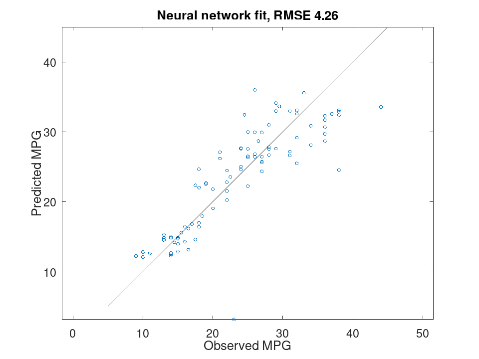
- Predict fuel economy from engine power and weight
 load carsmall
 X = [Horsepower, Weight];
 Mdl = fitrnet (X, MPG, 'Standardize', true, 'IterationLimit', 500);
Rows carrying a missing value were dropped, so ask about the ones used
 used = Mdl.RowsUsed;
 yFit = predict (Mdl, X(used,:));
 plot (MPG(used), yFit, 'o', [5, 45], [5, 45], 'k-');
 axis equal;
 xlabel ('Observed MPG');
 ylabel ('Predicted MPG');
 title (sprintf ('Neural network fit, RMSE %.2f', sqrt (resubLoss (Mdl))));
- Watching the fit converge
 load carsmall
 Mdl = fitrnet ([Horsepower, Weight], MPG, 'Standardize', true, ...
                'IterationLimit', 400);
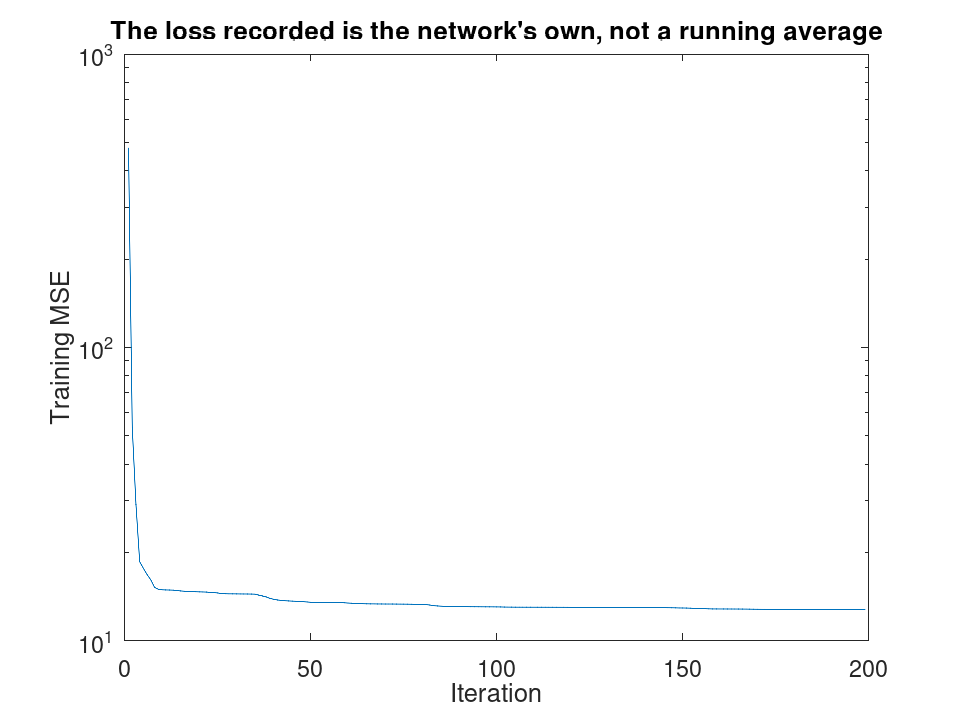
TrainingHistory records the mean squared error at every iteration
 h = Mdl.TrainingHistory;
 semilogy (h.Iteration, h.TrainingLoss, 'linewidth', 1.5);
 xlabel ('Iteration');
 ylabel ('Training MSE');
 title ('The loss recorded is the network''s own, not a running average');
- Standardizing matters when the predictors differ in scale
Horsepower runs to a few hundred and Weight to a few thousand, so the heavier column dominates the first layer until both are put on one scale.
 load carsmall
 X = [Horsepower, Weight];
 raw = fitrnet (X, MPG, 'IterationLimit', 400);
 std_ = fitrnet (X, MPG, 'Standardize', true, 'IterationLimit', 400);
 printf ('RMSE, raw predictors : %.2f\n', sqrt (resubLoss (raw)));
RMSE, raw predictors : 3.98
printf ('RMSE, standardized : %.2f\n', sqrt (resubLoss (std_)));
RMSE, standardized : 3.29
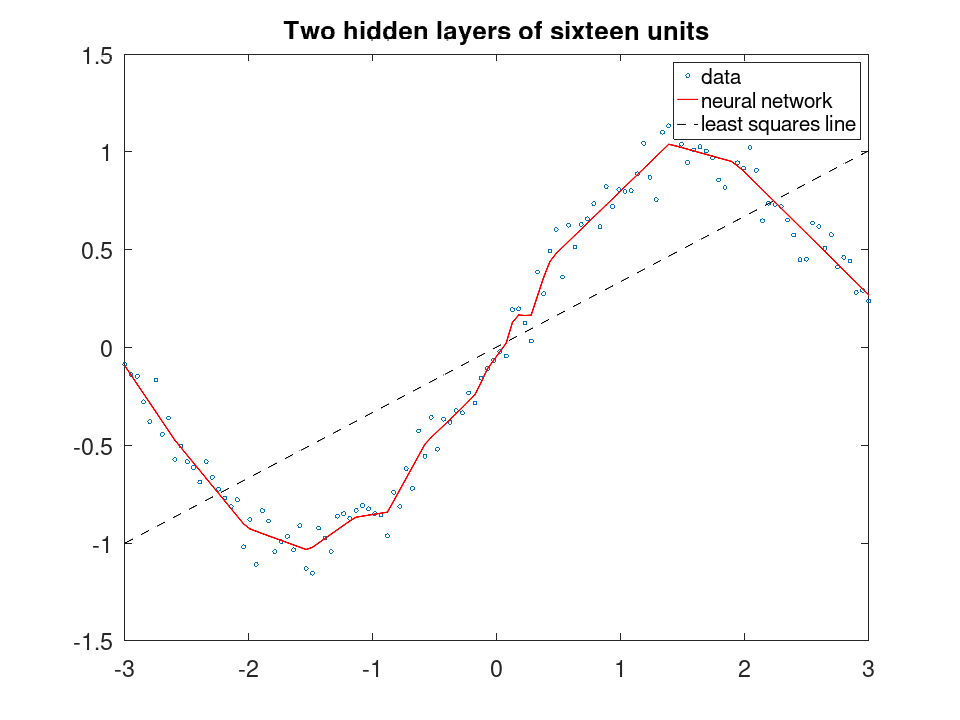
- A network recovers a curve a straight line cannot
 rng (42);
 x = linspace (-3, 3, 120)';
 y = sin (x) + randn (120, 1) * 0.1;
 Mdl = fitrnet (x, y, 'LayerSizes', [16, 16], 'IterationLimit', 800);
 plot (x, y, 'o', 'markersize', 4);
 hold on;
 plot (x, predict (Mdl, x), 'r-', 'linewidth', 2);
 plot (x, [ones(120,1), x] * ([ones(120,1), x] \ y), 'k--', 'linewidth', 1.5);
 hold off;
 legend ({'data', 'neural network', 'least squares line'});
 title ('Two hidden layers of sixteen units');
Fit from a table, and predict on one
 load fisheriris
 T = table (meas(:,2), meas(:,3), meas(:,4), meas(:,1), ...
            'VariableNames', {'SW', 'PL', 'PW', 'SL'});
 T.Wide = categorical (meas(:,2) > 3, [false true], {'narrow', 'wide'});
A model formula names the response and the predictors together, and holds main effects only
 Mdl = fitrnet (T, 'SL ~ PL + Wide');
 Mdl.PredictorNames
ans =
  1x2 cell array

    {'PL'}    {'Wide'}
Mdl.ResponseName
ans = SL
Mdl.CategoricalPredictors
ans = 2
predict matches the table's variables by name, so a column the model was not fitted on is passed over
 yFit = predict (Mdl, T(1:5,:));
 yFit'
ans =

   5.0283   4.6703   4.9826   5.0741   5.0283