Categories &
Functions List
- adtest
- anova
- anova1
- anova2
- anovan
- ansaribradley
- barttest
- binotest
- chi2gof
- chi2test
- correlation_test
- detectdrift
- dwtest
- fishertest
- friedman
- hotelling_t2test
- hotelling_t2test2
- jbtest
- knntest
- kruskalwallis
- kstest
- kstest2
- lillietest
- manova1
- mcnemar_test
- meanEffectSize
- mmdtest
- multcompare
- ranksum
- regression_ftest
- regression_ttest
- runstest
- signrank
- signtest
- stats.drift.DriftDiagnostics
- swtest
- ttest
- ttest2
- vartest
- vartest2
- vartestn
- ztest
- ztest2
- CompactLinearModel
- CoxModel
- coxphfit
- fitcox
- fitglm
- fitglme
- fitlm
- fitlme
- fitlmematrix
- fitnlm
- fitrm
- GeneralizedLinearMixedModel
- GeneralizedLinearModel
- glmfit
- glmval
- invpred
- lasso
- lassoglm
- LinearFormula
- LinearMixedModel
- LinearModel
- logistic_regression
- mnrfit
- mnrval
- monotone_smooth
- mvregress
- mvregresslike
- nlinfit
- nlparci
- nlpredci
- NonLinearModel
- plsregress
- regress
- regress_gp
- RepeatedMeasuresModel
- ridge
- robustfit
- stepwisefit
- stepwiseglm
- stepwiselm
- ClassificationBaggedEnsemble
- ClassificationDiscriminant
- ClassificationECOC
- ClassificationEnsemble
- ClassificationGAM
- ClassificationKernel
- ClassificationKNN
- ClassificationLinear
- ClassificationNaiveBayes
- ClassificationNeuralNetwork
- ClassificationPartitionedECOC
- ClassificationPartitionedEnsemble
- ClassificationPartitionedKernel
- ClassificationPartitionedLinear
- ClassificationPartitionedModel
- ClassificationSVM
- ClassificationTree
- CompactClassificationDiscriminant
- CompactClassificationECOC
- CompactClassificationEnsemble
- CompactClassificationGAM
- CompactClassificationNaiveBayes
- CompactClassificationNeuralNetwork
- CompactClassificationSVM
- CompactClassificationTree
- CompactRegressionGAM
- CompactRegressionEnsemble
- CompactRegressionGP
- CompactRegressionNeuralNetwork
- CompactRegressionSVM
- CompactRegressionTree
- CompactTreeBagger
- designecoc
- fcnnpredict
- fcnntrain
- fitcdiscr
- fitcecoc
- fitcensemble
- fitcgam
- fitckernel
- fitcknn
- fitclinear
- fitcnb
- fitcnet
- fitcsvm
- fitctree
- fitrensemble
- fitrgam
- fitrgp
- fitrkernel
- fitrlinear
- fitrnet
- fitrsvm
- fitrtree
- gamboostinter
- gamboostpairs
- gamboostpredict
- gamboosttrain
- gampredict
- gamtrain
- partialDependence
- plotPartialDependence
- PredictiveModel
- RegressionBaggedEnsemble
- RegressionEnsemble
- RegressionGAM
- RegressionGP
- RegressionKernel
- RegressionLinear
- RegressionNeuralNetwork
- RegressionPartitionedEnsemble
- RegressionPartitionedKernel
- RegressionPartitionedLinear
- RegressionPartitionedModel
- RegressionSVM
- RegressionTree
- lime
- shapley
- svmpredict
- svmtrain
- templateDiscriminant
- templateEnsemble
- templateKernel
- templateKNN
- templateLinear
- templateNaiveBayes
- templateSVM
- templateTree
- TreeBagger
- treepredict
- treetrain
- paretotails
- prob.ProbabilityDistribution
- prob.BetaDistribution
- prob.BinomialDistribution
- prob.BirnbaumSaundersDistribution
- prob.BurrDistribution
- prob.ExponentialDistribution
- prob.ExtremeValueDistribution
- prob.GammaDistribution
- prob.GeneralizedExtremeValueDistribution
- prob.GeneralizedParetoDistribution
- prob.HalfNormalDistribution
- prob.InverseGaussianDistribution
- prob.KernelDistribution
- prob.LogisticDistribution
- prob.LoglogisticDistribution
- prob.LognormalDistribution
- prob.LoguniformDistribution
- prob.MultinomialDistribution
- prob.NakagamiDistribution
- prob.NegativeBinomialDistribution
- prob.NormalDistribution
- prob.PiecewiseLinearDistribution
- prob.PoissonDistribution
- prob.RayleighDistribution
- prob.RicianDistribution
- prob.StableDistribution
- prob.tLocationScaleDistribution
- prob.TriangularDistribution
- prob.UniformDistribution
- prob.WeibullDistribution
- betafit
- betalike
- binofit
- binolike
- bisafit
- bisalike
- burrfit
- burrlike
- copulafit
- evfit
- evlike
- expfit
- explike
- gamfit
- gamlike
- geofit
- gevfit
- gevlike
- gevfit_lmom
- gpfit
- gplike
- gumbelfit
- gumbellike
- hnfit
- hnlike
- invgfit
- invglike
- logifit
- logilike
- loglfit
- logllike
- lognfit
- lognlike
- nakafit
- nakalike
- nbinfit
- nbinlike
- normfit
- normlike
- poissfit
- poisslike
- raylfit
- rayllike
- ricefit
- ricelike
- stblfit
- stbllike
- tlsfit
- tlslike
- unidfit
- unifit
- wblfit
- wbllike
- betacdf
- betainv
- betapdf
- betarnd
- binocdf
- binoinv
- binopdf
- binornd
- bisacdf
- bisainv
- bisapdf
- bisarnd
- burrcdf
- burrinv
- burrpdf
- burrrnd
- bvncdf
- bvtcdf
- cauchycdf
- cauchyinv
- cauchypdf
- cauchyrnd
- chi2cdf
- chi2inv
- chi2pdf
- chi2rnd
- copulacdf
- copulapdf
- copularnd
- evcdf
- evinv
- evpdf
- evrnd
- expcdf
- expinv
- exppdf
- exprnd
- fcdf
- finv
- fpdf
- frnd
- gamcdf
- gaminv
- gampdf
- gamrnd
- geocdf
- geoinv
- geopdf
- geornd
- gevcdf
- gevinv
- gevpdf
- gevrnd
- gpcdf
- gpinv
- gppdf
- gprnd
- gumbelcdf
- gumbelinv
- gumbelpdf
- gumbelrnd
- hncdf
- hninv
- hnpdf
- hnrnd
- hygecdf
- hygeinv
- hygepdf
- hygernd
- invgcdf
- invginv
- invgpdf
- invgrnd
- iwishpdf
- iwishrnd
- jsucdf
- jsupdf
- laplacecdf
- laplaceinv
- laplacepdf
- laplacernd
- logicdf
- logiinv
- logipdf
- logirnd
- loglcdf
- loglinv
- loglpdf
- loglrnd
- logncdf
- logninv
- lognpdf
- lognrnd
- mnpdf
- mnrnd
- mvncdf
- mvnpdf
- mvnrnd
- mvtcdf
- mvtpdf
- mvtrnd
- nakacdf
- nakainv
- nakapdf
- nakarnd
- nbincdf
- nbininv
- nbinpdf
- nbinrnd
- ncfcdf
- ncfinv
- ncfpdf
- ncfrnd
- nctcdf
- nctinv
- nctpdf
- nctrnd
- ncx2cdf
- ncx2inv
- ncx2pdf
- ncx2rnd
- normcdf
- norminv
- normpdf
- normrnd
- plcdf
- plinv
- plpdf
- plrnd
- poisscdf
- poissinv
- poisspdf
- poissrnd
- raylcdf
- raylinv
- raylpdf
- raylrnd
- ricecdf
- riceinv
- ricepdf
- ricernd
- stblcdf
- stblinv
- stblpdf
- stblrnd
- stdrcdf
- stdrinv
- stdrpdf
- stdrrnd
- tcdf
- tinv
- tpdf
- trnd
- tlscdf
- tlsinv
- tlspdf
- tlsrnd
- tricdf
- triinv
- tripdf
- trirnd
- unidcdf
- unidinv
- unidpdf
- unidrnd
- unifcdf
- unifinv
- unifpdf
- unifrnd
- vmcdf
- vminv
- vmpdf
- vmrnd
- wblcdf
- wblinv
- wblpdf
- wblrnd
- wienrnd
- wishpdf
- wishrnd
- betastat
- binostat
- bisastat
- burrstat
- chi2stat
- copulaparam
- copulastat
- evstat
- expstat
- fstat
- gamstat
- geostat
- gevstat
- gpstat
- gumbelstat
- hnstat
- hygestat
- invgstat
- logistat
- loglstat
- lognstat
- nakastat
- nbinstat
- ncfstat
- nctstat
- ncx2stat
- normstat
- plstat
- poisstat
- raylstat
- ricestat
- stdrstat
- tlsstat
- tristat
- tstat
- unidstat
- unifstat
- wblstat
- andrewsplot
- bar3
- bar3h
- biplot
- boxchart
- boxplot
- cdfplot
- dendrogram
- ecdfhist
- einstein
- gardnerAltmanPlot
- glyphplot
- gplotmatrix
- gscatter
- heatmap
- hist3
- histfit
- manovacluster
- normplot
- parallelcoords
- parallelplot
- ppplot
- probplot
- qqplot
- scatterhist
- scatterhistogram
- silhouette
- stats.chart.BoxChart
- stats.chart.HeatmapChart
- stats.chart.ParallelCoordinatesPlot
- stats.chart.ScatterHistogramChart
- swarmchart
- violin
- wblplot
Class Definition: shapley
statistics: shapley
Shapley values for a fitted model at one or more query points.
A Shapley value says how much one predictor contributed to the deviation of a prediction from the average prediction. The values of a query point sum to that deviation exactly, which is the property the computation is built to keep.
explainer = shapley (Mdl) builds an explainer for the
fitted model Mdl over the observations it was fitted on. A compact
model keeps none, so it must be given them as X, and so must a
function handle. Nothing is computed until query points are given, either
to the constructor as 'QueryPoints' or afterwards to
fit.
explainer = shapley (Mdl, X) takes the
observations to average over as X, a real numeric matrix of one
column per predictor.
X may also be a table, and so may 'QueryPoints' and what
fit is given. Where the model names its predictors the table is
read by those names and not by the order its columns come in, so a
column the model was not fitted on is passed over and a value holding a
level is coded as that level was coded at fitting. A function handle
names nothing, so a table given for one names the predictors itself and
its columns are taken in the order they come.
explainer = shapley (fun, X) takes a function
handle in place of a model. fun is called with a matrix of
observations and answers with one real numeric column holding one value
for each, so an explainer built on a handle always has a single column of
values.
| Name | Value | |
|---|---|---|
'QueryPoints' | The observations to explain, one per row, with one column per predictor. The default is none, which leaves the values unfitted. | |
'NumObservationsToSample' | How many observations to
draw, without replacement, from those averaged over, or 'all' for
every one of them. The default is 100, and so is any number reaching or
exceeding how many there are. A drawn sample makes the values differ from
one call to the next; 'all' is what makes them reproducible. | |
'CategoricalPredictors' | The predictors whose values are levels, taken as by every learner of this package. It applies only to a function handle, a model being asked for its own. | |
'MaxNumSubsets' | How many predictor subsets at most to compute over, an integer above 1. The default is the lesser of 2^M, which is every subset of the M predictors, and 1024. Every subset gives the values exactly; fewer estimates them, and fewer than 2M+2 estimates them poorly enough to warn about. Giving it at all asks for the subsets, so a linear model or a decision tree that would otherwise be answered from its own structure is answered over them instead. | |
'Method' | The algorithm, 'interventional'
by default, which averages over the observations as they stand.
'conditional' averages instead over the tenth of them lying
nearest the query point in the predictors being held, which stands in
for conditioning on those predictors. It asks more of the data and is
the dearer of the two. |
'UseParallel' is not implemented and is refused rather than
ignored.
See also: partialDependence, plotPartialDependence, PredictiveModel
Source Code: shapley
The shapley class contains the following properties:
The fitted model, or the function handle, the explainer was built on. This property is read-only.
Explain a model fitted from a table
 load fisheriris
 T = table (meas(:,2), meas(:,3), meas(:,4), meas(:,1), ...
            'VariableNames', {'SW', 'PL', 'PW', 'SL'});
 T.Wide = categorical (meas(:,2) > 3, [false true], {'narrow', 'wide'});
 Mdl = fitrtree (T, 'SL');
The observations and the query points may be tables too, read by the names the model was fitted on rather than by the order of the columns
 s = shapley (Mdl, T(:, [1, 2, 3, 5]), 'QueryPoints', T(1, [5, 3, 2, 1]), ...
              'NumObservationsToSample', 'all');
 s.Shapley
ans =
  4x2 table

    Predictor       Value
    _________    ___________

    "SW"            0.171493
    "PL"           -0.974986
    "PW"         -0.00650741
    "Wide"                 0
A column the model was not fitted on is passed over, so the whole table, response and all, gives the same explanation
 t = shapley (Mdl, T, 'QueryPoints', T(1,:), ...
              'NumObservationsToSample', 'all');
 isequal (t.Shapley.Value, s.Shapley.Value)
ans = 1
A real numeric matrix of one row per observation and one column per predictor, either given outright or taken from the model. It is the whole of what was given, before any sampling. This property is read-only.
Where the observations were given as a table, they are the coded matrix and not the table: a variable holding levels is stored as its level codes, and the coding is kept with the object.
Explain a model fitted from a table
 load fisheriris
 T = table (meas(:,2), meas(:,3), meas(:,4), meas(:,1), ...
            'VariableNames', {'SW', 'PL', 'PW', 'SL'});
 T.Wide = categorical (meas(:,2) > 3, [false true], {'narrow', 'wide'});
 Mdl = fitrtree (T, 'SL');
The observations and the query points may be tables too, read by the names the model was fitted on rather than by the order of the columns
 s = shapley (Mdl, T(:, [1, 2, 3, 5]), 'QueryPoints', T(1, [5, 3, 2, 1]), ...
              'NumObservationsToSample', 'all');
 s.Shapley
ans =
  4x2 table

    Predictor       Value
    _________    ___________

    "SW"            0.171493
    "PL"           -0.974986
    "PW"         -0.00650741
    "Wide"                 0
A column the model was not fitted on is passed over, so the whole table, response and all, gives the same explanation
 t = shapley (Mdl, T, 'QueryPoints', T(1,:), ...
              'NumObservationsToSample', 'all');
 isequal (t.Shapley.Value, s.Shapley.Value)
ans = 1
A real numeric matrix of one row per query point, empty until query points are given. This property is read-only.
Explain a model fitted from a table
 load fisheriris
 T = table (meas(:,2), meas(:,3), meas(:,4), meas(:,1), ...
            'VariableNames', {'SW', 'PL', 'PW', 'SL'});
 T.Wide = categorical (meas(:,2) > 3, [false true], {'narrow', 'wide'});
 Mdl = fitrtree (T, 'SL');
The observations and the query points may be tables too, read by the names the model was fitted on rather than by the order of the columns
 s = shapley (Mdl, T(:, [1, 2, 3, 5]), 'QueryPoints', T(1, [5, 3, 2, 1]), ...
              'NumObservationsToSample', 'all');
 s.Shapley
ans =
  4x2 table

    Predictor       Value
    _________    ___________

    "SW"            0.171493
    "PL"           -0.974986
    "PW"         -0.00650741
    "Wide"                 0
A column the model was not fitted on is passed over, so the whole table, response and all, gives the same explanation
 t = shapley (Mdl, T, 'QueryPoints', T(1,:), ...
              'NumObservationsToSample', 'all');
 isequal (t.Shapley.Value, s.Shapley.Value)
ans = 1
The response of a regression model or the predicted label of a classifier, one for each query point, empty until query points are given. A label keeps the type of the response the model was fitted with, as everywhere in this package. This property is read-only.
Explain a model fitted from a table
 load fisheriris
 T = table (meas(:,2), meas(:,3), meas(:,4), meas(:,1), ...
            'VariableNames', {'SW', 'PL', 'PW', 'SL'});
 T.Wide = categorical (meas(:,2) > 3, [false true], {'narrow', 'wide'});
 Mdl = fitrtree (T, 'SL');
The observations and the query points may be tables too, read by the names the model was fitted on rather than by the order of the columns
 s = shapley (Mdl, T(:, [1, 2, 3, 5]), 'QueryPoints', T(1, [5, 3, 2, 1]), ...
              'NumObservationsToSample', 'all');
 s.Shapley
ans =
  4x2 table

    Predictor       Value
    _________    ___________

    "SW"            0.171493
    "PL"           -0.974986
    "PW"         -0.00650741
    "Wide"                 0
A column the model was not fitted on is passed over, so the whole table, response and all, gives the same explanation
 t = shapley (Mdl, T, 'QueryPoints', T(1,:), ...
              'NumObservationsToSample', 'all');
 isequal (t.Shapley.Value, s.Shapley.Value)
ans = 1
A table of one row per predictor, holding the predictor names in
Predictor and the values in Value for a regression
model or a function handle, and in one variable per class, named after
it, for a classifier. Each such variable holds one column per query
point. It is empty until query points are given. This property is
read-only.
Explain a model fitted from a table
 load fisheriris
 T = table (meas(:,2), meas(:,3), meas(:,4), meas(:,1), ...
            'VariableNames', {'SW', 'PL', 'PW', 'SL'});
 T.Wide = categorical (meas(:,2) > 3, [false true], {'narrow', 'wide'});
 Mdl = fitrtree (T, 'SL');
The observations and the query points may be tables too, read by the names the model was fitted on rather than by the order of the columns
 s = shapley (Mdl, T(:, [1, 2, 3, 5]), 'QueryPoints', T(1, [5, 3, 2, 1]), ...
              'NumObservationsToSample', 'all');
 s.Shapley
ans =
  4x2 table

    Predictor       Value
    _________    ___________

    "SW"            0.171493
    "PL"           -0.974986
    "PW"         -0.00650741
    "Wide"                 0
A column the model was not fitted on is passed over, so the whole table, response and all, gives the same explanation
 t = shapley (Mdl, T, 'QueryPoints', T(1,:), ...
              'NumObservationsToSample', 'all');
 isequal (t.Shapley.Value, s.Shapley.Value)
ans = 1
A table laid out as Shapley, holding the mean over the query
points of the absolute values. With one query point it is their
absolute value. This property is read-only.
Explain a model fitted from a table
 load fisheriris
 T = table (meas(:,2), meas(:,3), meas(:,4), meas(:,1), ...
            'VariableNames', {'SW', 'PL', 'PW', 'SL'});
 T.Wide = categorical (meas(:,2) > 3, [false true], {'narrow', 'wide'});
 Mdl = fitrtree (T, 'SL');
The observations and the query points may be tables too, read by the names the model was fitted on rather than by the order of the columns
 s = shapley (Mdl, T(:, [1, 2, 3, 5]), 'QueryPoints', T(1, [5, 3, 2, 1]), ...
              'NumObservationsToSample', 'all');
 s.Shapley
ans =
  4x2 table

    Predictor       Value
    _________    ___________

    "SW"            0.171493
    "PL"           -0.974986
    "PW"         -0.00650741
    "Wide"                 0
A column the model was not fitted on is passed over, so the whole table, response and all, gives the same explanation
 t = shapley (Mdl, T, 'QueryPoints', T(1,:), ...
              'NumObservationsToSample', 'all');
 isequal (t.Shapley.Value, s.Shapley.Value)
ans = 1
The mean of what the model answers over the observations averaged over, a scalar for a regression model or a function handle and one value per class for a classifier. The values of a query point sum to the deviation of its prediction from this. This property is read-only.
Explain a model fitted from a table
 load fisheriris
 T = table (meas(:,2), meas(:,3), meas(:,4), meas(:,1), ...
            'VariableNames', {'SW', 'PL', 'PW', 'SL'});
 T.Wide = categorical (meas(:,2) > 3, [false true], {'narrow', 'wide'});
 Mdl = fitrtree (T, 'SL');
The observations and the query points may be tables too, read by the names the model was fitted on rather than by the order of the columns
 s = shapley (Mdl, T(:, [1, 2, 3, 5]), 'QueryPoints', T(1, [5, 3, 2, 1]), ...
              'NumObservationsToSample', 'all');
 s.Shapley
ans =
  4x2 table

    Predictor       Value
    _________    ___________

    "SW"            0.171493
    "PL"           -0.974986
    "PW"         -0.00650741
    "Wide"                 0
A column the model was not fitted on is passed over, so the whole table, response and all, gives the same explanation
 t = shapley (Mdl, T, 'QueryPoints', T(1,:), ...
              'NumObservationsToSample', 'all');
 isequal (t.Shapley.Value, s.Shapley.Value)
ans = 1
A character vector. 'interventional-linear' where the model
predicts a weighted sum of its predictors, which is answered from the
weights alone; 'interventional-tree' for a decision tree and
for an ensemble of them, which is answered leaf by leaf;
'interventional-kernel' for
every other model, which enumerates every subset of the predictors
where the budget allows it and estimates the values by weighted least
squares where it does not; and 'conditional-kernel' where
'Method' asked for conditioning. A tree and a linear model
are answered exactly however many predictors they have, where the
budget stops the subsets at 1024. This property is read-only.
Explain a model fitted from a table
 load fisheriris
 T = table (meas(:,2), meas(:,3), meas(:,4), meas(:,1), ...
            'VariableNames', {'SW', 'PL', 'PW', 'SL'});
 T.Wide = categorical (meas(:,2) > 3, [false true], {'narrow', 'wide'});
 Mdl = fitrtree (T, 'SL');
The observations and the query points may be tables too, read by the names the model was fitted on rather than by the order of the columns
 s = shapley (Mdl, T(:, [1, 2, 3, 5]), 'QueryPoints', T(1, [5, 3, 2, 1]), ...
              'NumObservationsToSample', 'all');
 s.Shapley
ans =
  4x2 table

    Predictor       Value
    _________    ___________

    "SW"            0.171493
    "PL"           -0.974986
    "PW"         -0.00650741
    "Wide"                 0
A column the model was not fitted on is passed over, so the whole table, response and all, gives the same explanation
 t = shapley (Mdl, T, 'QueryPoints', T(1,:), ...
              'NumObservationsToSample', 'all');
 isequal (t.Shapley.Value, s.Shapley.Value)
ans = 1
The lesser of what 'MaxNumSubsets' allowed and two raised to
the number of predictors, which is every subset. This property is
read-only.
Explain a model fitted from a table
 load fisheriris
 T = table (meas(:,2), meas(:,3), meas(:,4), meas(:,1), ...
            'VariableNames', {'SW', 'PL', 'PW', 'SL'});
 T.Wide = categorical (meas(:,2) > 3, [false true], {'narrow', 'wide'});
 Mdl = fitrtree (T, 'SL');
The observations and the query points may be tables too, read by the names the model was fitted on rather than by the order of the columns
 s = shapley (Mdl, T(:, [1, 2, 3, 5]), 'QueryPoints', T(1, [5, 3, 2, 1]), ...
              'NumObservationsToSample', 'all');
 s.Shapley
ans =
  4x2 table

    Predictor       Value
    _________    ___________

    "SW"            0.171493
    "PL"           -0.974986
    "PW"         -0.00650741
    "Wide"                 0
A column the model was not fitted on is passed over, so the whole table, response and all, gives the same explanation
 t = shapley (Mdl, T, 'QueryPoints', T(1,:), ...
              'NumObservationsToSample', 'all');
 isequal (t.Shapley.Value, s.Shapley.Value)
ans = 1
The indices of the predictors whose values are levels, empty where there are none. This property is read-only.
Explain a model fitted from a table
 load fisheriris
 T = table (meas(:,2), meas(:,3), meas(:,4), meas(:,1), ...
            'VariableNames', {'SW', 'PL', 'PW', 'SL'});
 T.Wide = categorical (meas(:,2) > 3, [false true], {'narrow', 'wide'});
 Mdl = fitrtree (T, 'SL');
The observations and the query points may be tables too, read by the names the model was fitted on rather than by the order of the columns
 s = shapley (Mdl, T(:, [1, 2, 3, 5]), 'QueryPoints', T(1, [5, 3, 2, 1]), ...
              'NumObservationsToSample', 'all');
 s.Shapley
ans =
  4x2 table

    Predictor       Value
    _________    ___________

    "SW"            0.171493
    "PL"           -0.974986
    "PW"         -0.00650741
    "Wide"                 0
A column the model was not fitted on is passed over, so the whole table, response and all, gives the same explanation
 t = shapley (Mdl, T, 'QueryPoints', T(1,:), ...
              'NumObservationsToSample', 'all');
 isequal (t.Shapley.Value, s.Shapley.Value)
ans = 1
A sorted column of indices into X, holding every row where
'NumObservationsToSample' did not draw a sample. This property
is read-only.
Explain a model fitted from a table
 load fisheriris
 T = table (meas(:,2), meas(:,3), meas(:,4), meas(:,1), ...
            'VariableNames', {'SW', 'PL', 'PW', 'SL'});
 T.Wide = categorical (meas(:,2) > 3, [false true], {'narrow', 'wide'});
 Mdl = fitrtree (T, 'SL');
The observations and the query points may be tables too, read by the names the model was fitted on rather than by the order of the columns
 s = shapley (Mdl, T(:, [1, 2, 3, 5]), 'QueryPoints', T(1, [5, 3, 2, 1]), ...
              'NumObservationsToSample', 'all');
 s.Shapley
ans =
  4x2 table

    Predictor       Value
    _________    ___________

    "SW"            0.171493
    "PL"           -0.974986
    "PW"         -0.00650741
    "Wide"                 0
A column the model was not fitted on is passed over, so the whole table, response and all, gives the same explanation
 t = shapley (Mdl, T, 'QueryPoints', T(1,:), ...
              'NumObservationsToSample', 'all');
 isequal (t.Shapley.Value, s.Shapley.Value)
ans = 1
The shapley class offers the following public methods:
shapley: obj = shapley (Mdl)
shapley: obj = shapley (Mdl, X)
shapley: obj = shapley (fun, X)
shapley: obj = shapley (…, name, value)
The arguments are those described for the class. Where
'QueryPoints' is given the values are computed at once,
otherwise they are left to fit.
See also: shapley, shapley.fit
Explain a model fitted from a table
 load fisheriris
 T = table (meas(:,2), meas(:,3), meas(:,4), meas(:,1), ...
            'VariableNames', {'SW', 'PL', 'PW', 'SL'});
 T.Wide = categorical (meas(:,2) > 3, [false true], {'narrow', 'wide'});
 Mdl = fitrtree (T, 'SL');
The observations and the query points may be tables too, read by the names the model was fitted on rather than by the order of the columns
 s = shapley (Mdl, T(:, [1, 2, 3, 5]), 'QueryPoints', T(1, [5, 3, 2, 1]), ...
              'NumObservationsToSample', 'all');
 s.Shapley
ans =
  4x2 table

    Predictor       Value
    _________    ___________

    "SW"            0.171493
    "PL"           -0.974986
    "PW"         -0.00650741
    "Wide"                 0
A column the model was not fitted on is passed over, so the whole table, response and all, gives the same explanation
 t = shapley (Mdl, T, 'QueryPoints', T(1,:), ...
              'NumObservationsToSample', 'all');
 isequal (t.Shapley.Value, s.Shapley.Value)
ans = 1
shapley: obj = fit (obj, QueryPoints)
QueryPoints is a real numeric matrix of one row per query point and one column per predictor, or a table read by the names the explainer holds. The values already held are replaced, not added to.
See also: shapley
Explain a model fitted from a table
 load fisheriris
 T = table (meas(:,2), meas(:,3), meas(:,4), meas(:,1), ...
            'VariableNames', {'SW', 'PL', 'PW', 'SL'});
 T.Wide = categorical (meas(:,2) > 3, [false true], {'narrow', 'wide'});
 Mdl = fitrtree (T, 'SL');
The observations and the query points may be tables too, read by the names the model was fitted on rather than by the order of the columns
 s = shapley (Mdl, T(:, [1, 2, 3, 5]), 'QueryPoints', T(1, [5, 3, 2, 1]), ...
              'NumObservationsToSample', 'all');
 s.Shapley
ans =
  4x2 table

    Predictor       Value
    _________    ___________

    "SW"            0.171493
    "PL"           -0.974986
    "PW"         -0.00650741
    "Wide"                 0
A column the model was not fitted on is passed over, so the whole table, response and all, gives the same explanation
 t = shapley (Mdl, T, 'QueryPoints', T(1,:), ...
              'NumObservationsToSample', 'all');
 isequal (t.Shapley.Value, s.Shapley.Value)
ans = 1
shapley: plot (obj)
shapley: plot (obj, name, value)
shapley: plot (ax, …)
shapley: b = plot (…)
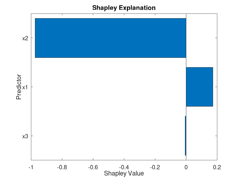
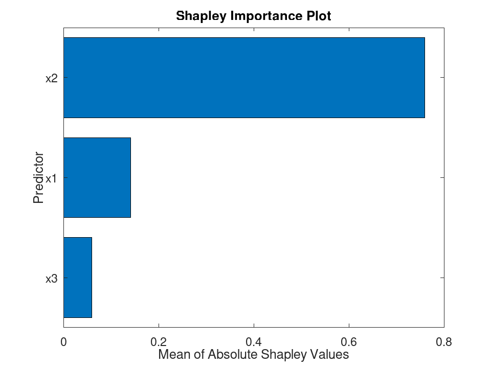
One bar per predictor, the least important at the bottom. Over one
query point the bars hold the values themselves and the chart is
titled 'Shapley Explanation'; over several they hold the mean
of the absolute values and it is titled
'Shapley Importance Plot'.
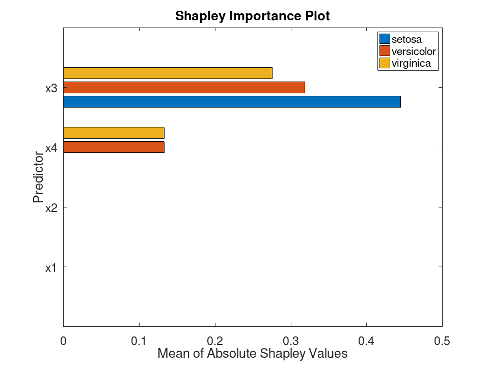
ax is the axes to draw into, the current one where none is given. b holds one bar series per class drawn.
| Name | Value | |
|---|---|---|
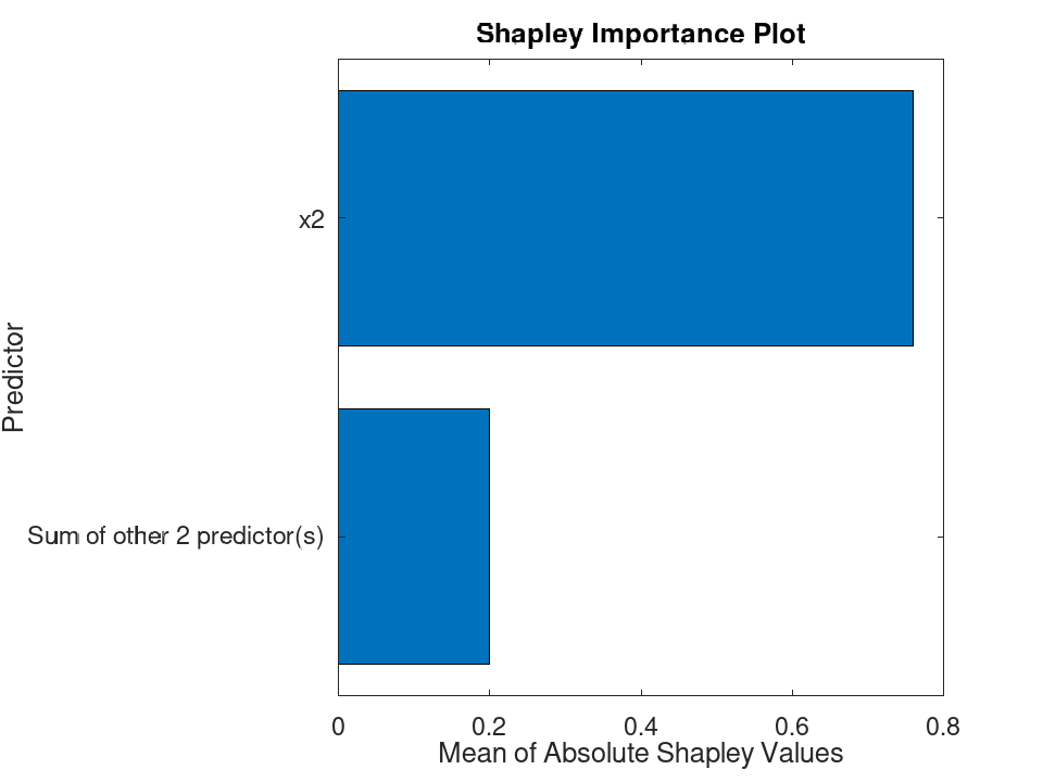
'NumImportantPredictors' | How many predictors to draw on their own, the ten most important by default. Over several query points whatever is left over is drawn as one further bar holding its sum; over one query point it is left out. | |
'ClassNames' | The classes to draw, for a classification model. The default is the predicted class over one query point and every class over several. | |
'QueryPointIndices' | Which query points to draw, all of them by default. |
See also: shapley, shapley.boxchart, shapley.swarmchart
- Explaining one prediction
 load fisheriris
 mdl = fitrtree (meas(:,2:4), meas(:,1));
 s = shapley (mdl, 'QueryPoints', meas(1,2:4), ...
              'NumObservationsToSample', 'all');
One value per predictor, summing to the deviation of the prediction from the average prediction
s.Shapley
ans =
  3x2 table

    Predictor       Value
    _________    ___________

    "x1"            0.171493
    "x2"           -0.974986
    "x3"         -0.00650741
A bar per predictor, the most important at the top
plot (s);
- Which predictors matter over many points
 load fisheriris
 mdl = fitrtree (meas(:,2:4), meas(:,1));
 s = shapley (mdl, 'QueryPoints', meas(1:5:150,2:4), ...
              'NumObservationsToSample', 'all');
Over several query points the bars hold the mean of the absolute values, so the chart reads as an importance plot rather than as an explanation of any one point
plot (s);
- The lesser predictors gathered into one bar
 load fisheriris
 mdl = fitrtree (meas(:,2:4), meas(:,1));
 s = shapley (mdl, 'QueryPoints', meas(1:5:150,2:4), ...
              'NumObservationsToSample', 'all');
Whatever NumImportantPredictors leaves out is summed into one further bar, so nothing goes missing from the picture
plot (s, 'NumImportantPredictors', 1);
- A classifier is explained one class at a time
 load fisheriris
 mdl = fitctree (meas, species);
 s = shapley (mdl, 'QueryPoints', meas([1, 60, 120],:), ...
              'NumObservationsToSample', 'all');
Over several query points every class is drawn, in the model's own order, and a legend names them
plot (s);
shapley: boxchart (obj)
shapley: boxchart (obj, name, value)
shapley: boxchart (ax, …)
shapley: b = boxchart (…)
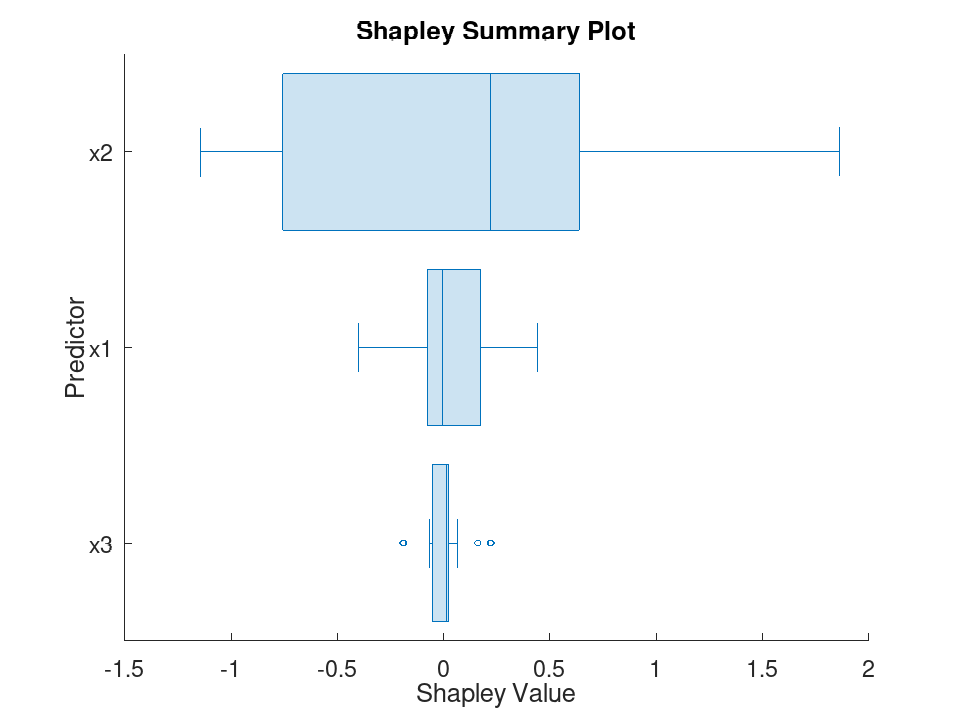
One box per predictor, the least important at the bottom, spread over
the query points the values were fitted at. The chart is titled
'Shapley Summary Plot' and lies horizontally.
ax is the axes to draw into, the current one where none is
given. b is the stats.chart.BoxChart drawn.
| Name | Value | |
|---|---|---|
'NumImportantPredictors' | How many predictors to draw, the ten most important by default. Whatever is left over is left out rather than summed, a box over a sum meaning nothing. | |
'ClassName' | The one class to draw, for a classification model. The default is the first class of the model. | |
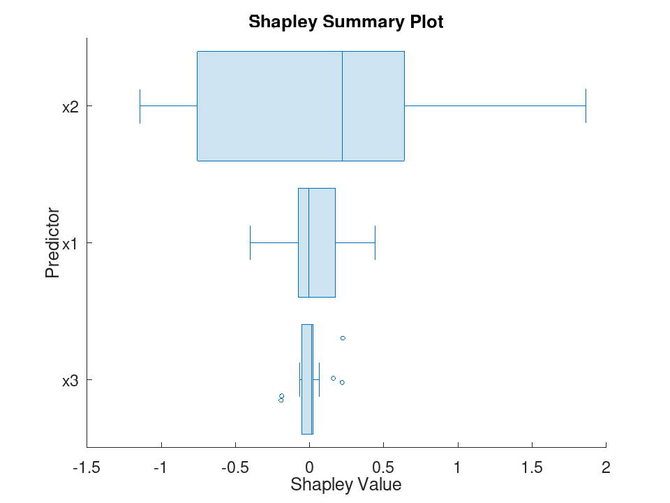
'JitterOutliers' | Whether outlier markers are
spread across the width of the box, 'off' by default. |
See also: shapley, shapley.plot, shapley.swarmchart, stats.chart.BoxChart
- How widely a predictor's contribution varies
 load fisheriris
 mdl = fitrtree (meas(:,2:4), meas(:,1));
 s = shapley (mdl, 'QueryPoints', meas(1:5:150,2:4), ...
              'NumObservationsToSample', 'all');
One box per predictor over the query points: the box spans the quartiles, and a predictor whose box is wide contributes differently from one point to the next
boxchart (s);
- The values that lie beyond the whiskers
 load fisheriris
 mdl = fitrtree (meas(:,2:4), meas(:,1));
 s = shapley (mdl, 'QueryPoints', meas(1:5:150,2:4), ...
              'NumObservationsToSample', 'all');
JitterOutliers spreads the outlier markers across the width of the box rather than drawing them in a line, so points at the same value stop hiding one another
boxchart (s, 'JitterOutliers', 'on');
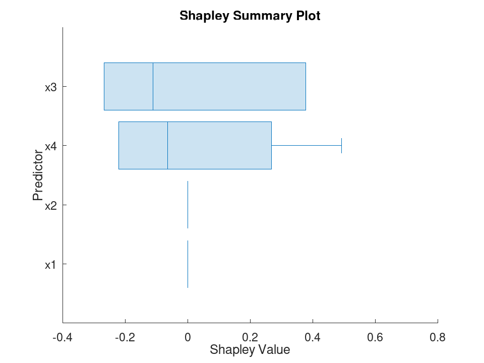
- One class of a classifier
 load fisheriris
 mdl = fitctree (meas, species);
 s = shapley (mdl, 'QueryPoints', meas(1:5:150,:), ...
              'NumObservationsToSample', 'all');
A box chart draws one class at a time, the first of them where none is named, and orders the predictors by that class
boxchart (s, 'ClassName', 'virginica');
shapley: swarmchart (obj)
shapley: swarmchart (obj, name, value)
shapley: swarmchart (ax, …)
shapley: s = swarmchart (…)
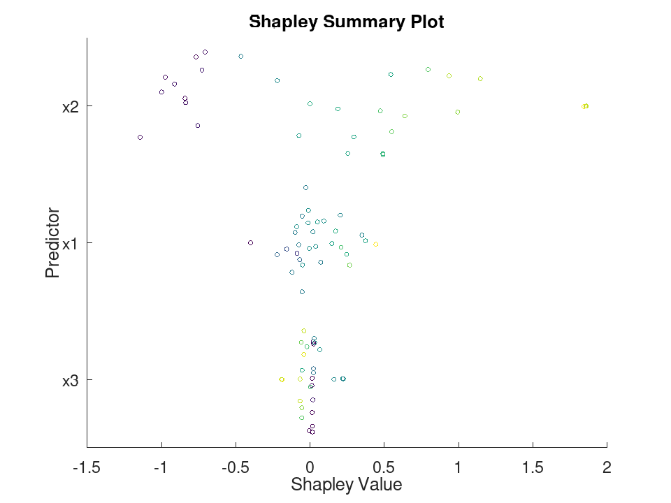
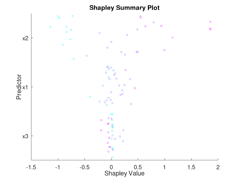
One row of points per predictor, the least important at the bottom,
one point per query point spread vertically by how crowded its
neighbourhood is. Each point is coloured by the value the predictor
takes at that query point, the least of them at one end of the
colour map and the greatest at the other. The chart is titled
'Shapley Summary Plot'.
ax is the axes to draw into, the current one where none is given. s holds one scatter object per predictor drawn.
| Name | Value | |
|---|---|---|
'NumImportantPredictors' | How many predictors to draw, the ten most important by default. | |
'ClassName' | The one class to draw, for a classification model. The default is the first class of the model. | |
'YJitter' | How the points of a row are spread,
'density' by default, or 'rand', 'randn' or
'none'. | |
'ColorMap' | The colour map the predictor values are read through, as a name or as a matrix of one RGB triplet per row. The default is the one the axes already carries. |
See also: shapley, shapley.plot, shapley.boxchart, swarmchart
- Every query point, coloured by the predictor's own value
 load fisheriris
 mdl = fitrtree (meas(:,2:4), meas(:,1));
 s = shapley (mdl, 'QueryPoints', meas(1:5:150,2:4), ...
              'NumObservationsToSample', 'all');
One point per query point per predictor, spread by how crowded its neighbourhood is. Colour says where the predictor's value stands in its own range, so a row whose colours run from one end to the other shows the contribution following the predictor
swarmchart (s);
- Choosing the colours and the spreading
 load fisheriris
 mdl = fitrtree (meas(:,2:4), meas(:,1));
 s = shapley (mdl, 'QueryPoints', meas(1:5:150,2:4), ...
              'NumObservationsToSample', 'all');
ColorMap takes a name or a matrix of RGB triplets, and YJitter takes 'rand' where an even spread reads better than a dense one
swarmchart (s, 'ColorMap', 'cool', 'YJitter', 'rand');
- One class of a classifier
 load fisheriris
 mdl = fitctree (meas, species);
 s = shapley (mdl, 'QueryPoints', meas(1:5:150,:), ...
              'NumObservationsToSample', 'all');
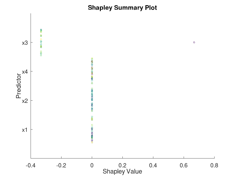
As for a box chart, one class is drawn at a time
swarmchart (s, 'ClassName', 'setosa');
shapley: plotDependence (obj, predictor)
shapley: plotDependence (obj, predictor, name, value)
shapley: plotDependence (ax, …)
shapley: p = plotDependence (…)
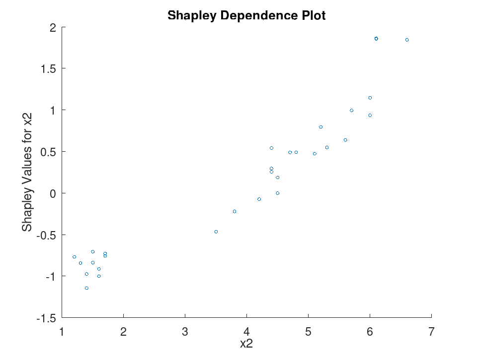
predictor names or indexes the predictor. Where it holds numbers the chart is a scatter of its value at each query point against the value it was given there; where it holds levels the chart is a box of the values at each level.
The chart is titled 'Shapley Dependence Plot' and its
vertical axis is labelled after the predictor drawn.
ax is the axes to draw into, the current one where none is
given. p is the scatter object, or the
stats.chart.BoxChart, drawn.
| Name | Value | |
|---|---|---|
'ClassName' | The one class to draw, for a classification model. The default is the first class of the model. | |
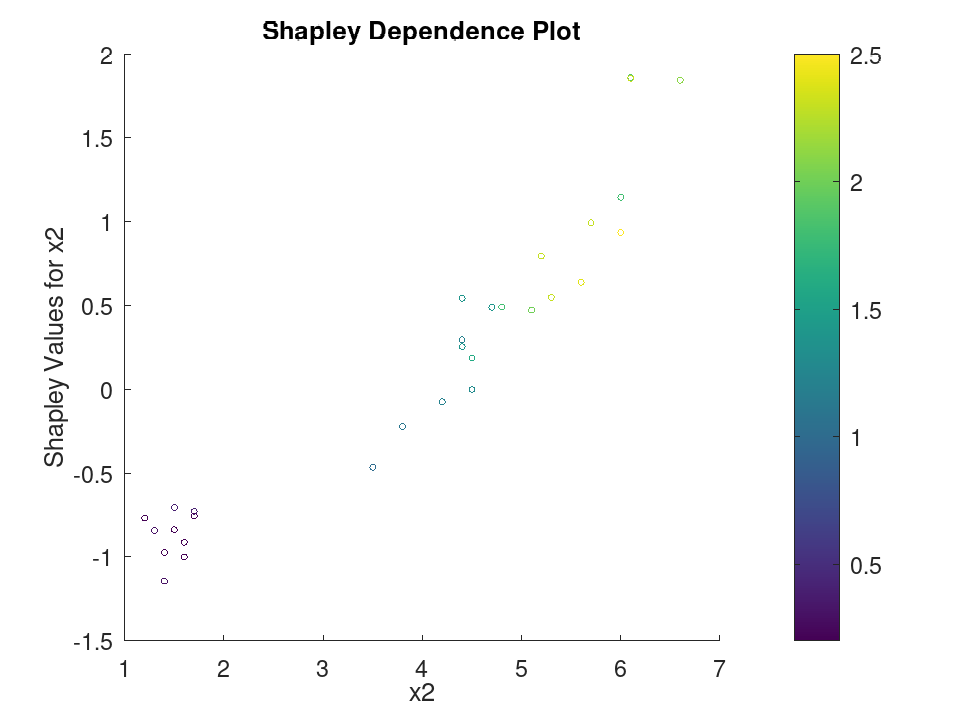
'ColorPredictor' | A second predictor to colour the points by, none by default. Its values are read as they stand, the range of the axes carrying the scale, and a colour bar is drawn beside the chart. It applies only where the predictor drawn holds numbers. | |
'ColorMap' | The colour map the colouring predictor is read through, as a name or as a matrix of one RGB triplet per row. The default is the one the axes already carries. |
See also: shapley, shapley.plot, shapley.swarmchart
- A predictor's contribution against its own value
 load fisheriris
 mdl = fitrtree (meas(:,2:4), meas(:,1));
 s = shapley (mdl, 'QueryPoints', meas(1:5:150,2:4), ...
              'NumObservationsToSample', 'all');
One point per query point: the predictor's value across, its Shapley value up. A rising cloud says the predictor pushes the prediction up the larger it gets
plotDependence (s, 'x2');
- A second predictor brought in as colour
 load fisheriris
 mdl = fitrtree (meas(:,2:4), meas(:,1));
 s = shapley (mdl, 'QueryPoints', meas(1:5:150,2:4), ...
              'NumObservationsToSample', 'all');
ColorPredictor colours each point by another predictor's value and draws a colour bar for the scale, which is how an interaction between the two shows itself
plotDependence (s, 'x2', 'ColorPredictor', 'x3');
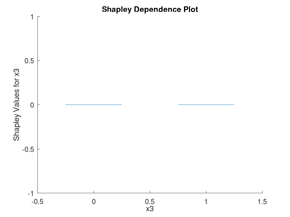
- A predictor holding levels
 load fisheriris
 X = [meas(:,2:3), double(strcmp (species, 'setosa'))];
 mdl = fitrtree (X, meas(:,1), 'CategoricalPredictors', 3);
 s = shapley (mdl, 'QueryPoints', X(1:5:150,:), ...
              'NumObservationsToSample', 'all');
Where the predictor holds levels rather than numbers the chart is a box over each level instead of a scatter
plotDependence (s, 'x3');
Examples
 load fisheriris
 T = table (meas(:,2), meas(:,3), meas(:,4), meas(:,1), ...
            'VariableNames', {'SW', 'PL', 'PW', 'SL'});
 T.Wide = categorical (meas(:,2) > 3, [false true], {'narrow', 'wide'});
 Mdl = fitrtree (T, 'SL');
The observations and the query points may be tables too, read by the names the model was fitted on rather than by the order of the columns
 s = shapley (Mdl, T(:, [1, 2, 3, 5]), 'QueryPoints', T(1, [5, 3, 2, 1]), ...
              'NumObservationsToSample', 'all');
 s.Shapley
ans =
  4x2 table

    Predictor       Value
    _________    ___________

    "SW"            0.171493
    "PL"           -0.974986
    "PW"         -0.00650741
    "Wide"                 0
A column the model was not fitted on is passed over, so the whole table, response and all, gives the same explanation
 t = shapley (Mdl, T, 'QueryPoints', T(1,:), ...
              'NumObservationsToSample', 'all');
 isequal (t.Shapley.Value, s.Shapley.Value)
ans = 1