The table the model was fitted to, one row per subject, responses included. A subject missing a response or a predictor is kept here, although the fit leaves it out. This property is read-only.

A character vector holding the right side of the model formula, with its intercept, as in '1 + species'. This property is read-only.

A cell row of character vectors naming the variables the between-subject model draws on, empty for a model with an intercept alone. This property is read-only.

A cell row of character vectors naming the repeated measures, in the order of the columns of Coefficients. This property is read-only.

A table with one row per response, named by the responses, and one variable per within-subject factor. Without a design given at fitting it holds a single factor Time of the values 1 to k for k responses. This property is read-only.

'separatemeans', 'orthogonalcontrasts', a formula over the within-subject factors or a contrast matrix, as given at fitting. This property is read-only.

A cell row of character vectors, the variable names of WithinDesign. This property is read-only.

A table with one row per coefficient, named after the terms of the between-subject model, and one variable per response. This property is read-only.

A table holding the covariance of the residuals of the responses, their cross products over DFE, with rows and variables named by the responses. This property is read-only.

The number of subjects the fit used less the number of between-subject coefficients. This property is read-only.

RepeatedMeasuresModel: rm = RepeatedMeasuresModel (t, modelspec)

RepeatedMeasuresModel: rm = RepeatedMeasuresModel (t, modelspec, name, value)

rm = RepeatedMeasuresModel (t, modelspec) fits the repeated measures in the table t on the between-subject model given by the formula modelspec, a character vector or a string scalar of the form 'responses ~ terms'. The responses are a range of the table’s variables, as in 'y1-y6', which takes every variable from y1 to y6 in the table’s order, a comma list, as in 'y1,y2,y3', or both. The terms are a Wilkinson formula over the other variables, as in 'species' or 'g*x', or '1' for an intercept alone. A categorical, logical, text or string variable is a categorical predictor and any other a continuous one.

A subject missing a response or a predictor is left out of the fit.

The following name-value arguments are accepted.

'orthogonalcontrasts' is refused at fitting unless the within-subject design holds a single numeric factor. MATLAB accepts the fit and refuses the model only when a test is asked of it.

See also: fitrm

RepeatedMeasuresModel: tbl = ranova (rm)

RepeatedMeasuresModel: tbl = ranova (rm, 'WithinModel', WM)

RepeatedMeasuresModel: [tbl, A, C, D] = ranova (…)

tbl = ranova (rm) tests the within-subject effects of the repeated measures model rm: whether the means of the responses differ, and whether each between-subject term changes that difference. tbl holds one row per test and one per error term, with the variables SumSq, DF, MeanSq, F and pValue, and beside them the p-values under the Greenhouse-Geisser, Huynh-Feldt and lower bound corrections for departures from sphericity, pValueGG, pValueHF and pValueLB. The corrections are reported and never applied.

ranova (rm, 'WithinModel', WM) tests the within-subject model WM instead, which takes the forms the 'WithinModel' argument of fitrm takes. The default is 'separatemeans' whatever the model was fitted with, as in MATLAB. Under 'separatemeans' or a contrast matrix the rows are named after the within-subject factor, or Time when there are several. A formula or 'orthogonalcontrasts' gives one block of rows per within-subject term, the constant term first, whose tests are the between-subject tests of the mean of the responses.

[tbl, A, C, D] = ranova (…) also returns the hypothesis of each test as A B C = D: A a cell column holding the between-subject hypothesis matrix of each term, C the within-subject contrast, a cell row of one per term when there are several, and D zero.

'orthogonalcontrasts' works here where MATLAB R2024a and R2026a both fail inside ranova; its results agree with those of MATLAB’s anova for the same contrasts.

See also: fitrm, RepeatedMeasuresModel.epsilon, RepeatedMeasuresModel.mauchly

 load fisheriris
 t = table (species, meas(:,1), meas(:,2), meas(:,3), meas(:,4), ...
            'VariableNames', {'species', 'meas1', 'meas2', 'meas3', 'meas4'});
 Meas = table ([1, 2, 3, 4]', 'VariableNames', {'Measurements'});
 rm = fitrm (t, 'meas1-meas4 ~ species', 'WithinDesign', Meas);

 ranova (rm)

ans =
  3x8 table

                                 SumSq     DF      MeanSq         F          pValue         pValueGG        pValueHF        pValueLB      
                                _______    ___    _________    _______    ____________    ____________    ____________    ____________    

    (Intercept):Measurements    1656.26      3      552.088    6873.29               0    9.44912e-279     2.9213e-283    2.58715e-125    
    species:Measurements        282.466      6      47.0777      586.1    1.42714e-206    4.93131e-156    1.54056e-158     9.01515e-71    
    Error(Measurements)         35.4227    441    0.0803237        NaN             NaN             NaN             NaN             NaN

 mauchly (rm)

ans =
  1x4 table

       W        ChiStat    DF      pValue       
    ________    _______    __    ___________    

    0.558144    84.9762     5    7.61488e-17

 epsilon (rm)

ans =
  1x4 table

    Uncorrected    GreenhouseGeisser    HuynhFeldt    LowerBound    
    ___________    _________________    __________    __________    

              1              0.75179      0.764092      0.333333

 load fisheriris
 t = table (species, meas(:,1), meas(:,2), meas(:,3), meas(:,4), ...
            'VariableNames', {'species', 'meas1', 'meas2', 'meas3', 'meas4'});
 Meas = table ([1, 2, 3, 4]', 'VariableNames', {'Measurements'});
 rm = fitrm (t, 'meas1-meas4 ~ species', 'WithinDesign', Meas);

 ranova (rm, 'WithinModel', 'orthogonalcontrasts')

ans =
  12x8 table

                                   SumSq      DF      MeanSq         F          pValue         pValueGG        pValueHF        pValueLB      
                                  ________    ___    _________    _______    ____________    ____________    ____________    ____________    

    (Intercept)                    7201.66      1      7201.66    19650.1    2.07354e-158    2.07354e-158    2.07354e-158    2.07354e-158    
    species                        309.607      2      154.803     422.39     1.15165e-61     1.15165e-61     1.15165e-61     1.15165e-61    
    Error                          53.8746    147     0.366494        NaN             NaN             NaN             NaN             NaN    
    (Intercept):Measurements       1313.01      1      1313.01    14029.1    9.51133e-148    9.51133e-148    9.51133e-148    9.51133e-148    
    species:Measurements           35.9781      2       17.989    192.207     9.51777e-42     9.51777e-42     9.51777e-42     9.51777e-42    
    Error(Measurements)             13.758    147    0.0935922        NaN             NaN             NaN             NaN             NaN    
    (Intercept):Measurements^2     1.93802      1      1.93802    62.7528     5.31247e-13     5.31247e-13     5.31247e-13     5.31247e-13    
    species:Measurements^2        0.469633      2     0.234817    7.60335     0.000720725     0.000720725     0.000720725     0.000720725    
    Error(Measurements^2)          4.53985    147    0.0308833        NaN             NaN             NaN             NaN             NaN    
    (Intercept):Measurements^3     341.314      1      341.314    2929.84     5.62469e-99     5.62469e-99     5.62469e-99     5.62469e-99    
    species:Measurements^3         246.019      2      123.009    1055.91     6.12904e-88     6.12904e-88     6.12904e-88     6.12904e-88    
    Error(Measurements^3)          17.1248    147     0.116496        NaN             NaN             NaN             NaN             NaN

RepeatedMeasuresModel: tbl = epsilon (rm)

RepeatedMeasuresModel: tbl = epsilon (rm, C)

tbl = epsilon (rm) returns the corrections for departures from sphericity that ranova applies to its p-values, over the contrasts between successive responses: the variables Uncorrected, which is 1, GreenhouseGeisser, HuynhFeldt and LowerBound. The Huynh-Feldt value is Lecoutre’s corrected form, capped at 1, and the lower bound is 1 / p for p contrasts.

tbl = epsilon (rm, C) computes them over the contrast matrix C, which must have one row per response.

See also: fitrm, RepeatedMeasuresModel.ranova, RepeatedMeasuresModel.mauchly

RepeatedMeasuresModel: tbl = mauchly (rm)

RepeatedMeasuresModel: tbl = mauchly (rm, C)

tbl = mauchly (rm) tests whether the covariance of the contrasts between successive responses is a multiple of the identity, the sphericity that the uncorrected p-values of ranova assume. tbl holds Mauchly’s W, the chi-square statistic ChiStat with Bartlett’s factor, its degrees of freedom DF and the pValue. A singular covariance gives W 0, ChiStat Inf and a p-value of 0.

tbl = mauchly (rm, C) tests the contrasts of the matrix C, which must have one row per response.

See also: fitrm, RepeatedMeasuresModel.ranova, RepeatedMeasuresModel.epsilon

RepeatedMeasuresModel: tbl = anova (rm)

RepeatedMeasuresModel: tbl = anova (rm, 'WithinModel', WM)

tbl = anova (rm) tests the between-subject terms of the repeated measures model rm on the average of the repeated measures, one univariate analysis of variance. tbl has the variables Within, the within-subject response analysed, Between, the between-subject term tested or Error, SumSq, DF, MeanSq, F and pValue. The intercept is named constant.

anova (rm, 'WithinModel', WM) analyses other responses built from the repeated measures, one block of rows each:

• 'separatemeans', the default: the average, named Constant.
• 'orthogonalcontrasts': the average and the orthogonal polynomial trends over a single numeric within-subject factor.
• A formula over the within-subject factors: each column of its effects-coded design, scaled to unit length and named after it.
• A contrast matrix with one row per response: each column as given, named Contrast1, Contrast2, …

MATLAB R2024a and R2026a fail on 'separatemeans' given explicitly, though it is their documented default; here it is the default.

See also: fitrm, RepeatedMeasuresModel.ranova, RepeatedMeasuresModel.manova

RepeatedMeasuresModel: tbl = manova (rm)

RepeatedMeasuresModel: tbl = manova (rm, name, value)

RepeatedMeasuresModel: [tbl, A, C, D] = manova (…)

tbl = manova (rm) tests every term of the within-subject model of rm, as it was fitted, against every between-subject term, by the four multivariate statistics. tbl has the variables Within, Between, Statistic, one of Pillai, Wilks, Hotelling and Roy, its Value, the F statistic that approximates it, RSquare, the degrees of freedom df1 and df2, and the pValue. Under 'separatemeans' the within-subject hypothesis is that of equal means, named Constant, and a contrast matrix is named Specified contrast.

The name-value arguments are 'WithinModel', which takes the forms fitrm takes but 'orthogonalcontrasts', and 'By', the name of a between-subject factor, which tests the within-subject hypotheses at each of its levels in place of the between-subject terms.

[tbl, A, C, D] = manova (…) also returns the hypotheses as A B C = D: A a cell column of the between-subject hypothesis matrices, C the within-subject contrast, a cell row of one per term when there are several, and D zero.

Pillai’s trace, Wilks’ lambda and Roy’s root are approximated by F as in MATLAB. The Hotelling-Lawley trace uses McKeon’s F approximation with its own second degrees of freedom, as SAS does, and the Pillai-Samson one where McKeon’s is undefined. MATLAB R2024a computes McKeon’s F but refers it to the Pillai-Samson degrees of freedom, which makes its p-values too small.

See also: fitrm, RepeatedMeasuresModel.coeftest, RepeatedMeasuresModel.ranova

RepeatedMeasuresModel: tbl = coeftest (rm, A, C)

RepeatedMeasuresModel: tbl = coeftest (rm, A, C, D)

tbl = coeftest (rm, A, C) tests the hypothesis A B C = 0 on the coefficient matrix B of rm, A having one column per between-subject coefficient and C one row per response. tbl holds the four multivariate statistics as manova reports them: the variables Statistic, Value, F, RSquare, df1, df2 and pValue.

tbl = coeftest (rm, A, C, D) tests A B C = D instead, D a scalar or a matrix with as many rows as A and as many columns as C. The default is 0.

See also: fitrm, RepeatedMeasuresModel.manova

RepeatedMeasuresModel: tbl = margmean (rm, vars)

RepeatedMeasuresModel: tbl = margmean (rm, vars, 'Alpha', alpha)

tbl = margmean (rm, vars) estimates the mean of the repeated measures at each combination of the levels of the factors named by vars, a character vector or a cell array of them, each a categorical between-subject factor or a within-subject factor. The other between-subject factors are averaged over their levels with equal weights, a continuous predictor is held at its mean over the subjects the fit used, and the responses are averaged over the other within-subject factors. tbl holds one variable per factor, the first varying slowest, and Mean, StdErr, Lower and Upper, the limits of a 100 (1 - alpha) per cent confidence interval on DFE degrees of freedom. The default alpha is 0.05.

See also: fitrm, RepeatedMeasuresModel.multcompare, RepeatedMeasuresModel.grpstats

RepeatedMeasuresModel: tbl = grpstats (rm, g)

RepeatedMeasuresModel: tbl = grpstats (rm, g, stats)

tbl = grpstats (rm, g) pools the repeated measures of every subject and summarizes them at each combination of the levels of the factors named by g, a character vector or a cell array of them, each a categorical between-subject factor or a within-subject factor. tbl holds one variable per factor, GroupCount, the number of values in the group, and their mean and std.

tbl = grpstats (rm, g, stats) computes the statistics named by stats instead, a character vector or a cell array of them, each one of 'mean', 'median', 'std', 'var', 'sem', 'min', 'max', 'range' and 'numel'. Missing values are left out.

See also: fitrm, RepeatedMeasuresModel.margmean

RepeatedMeasuresModel: tbl = multcompare (rm, var)

RepeatedMeasuresModel: tbl = multcompare (rm, var, name, value)

tbl = multcompare (rm, var) compares the estimated marginal means of every pair of levels of the factor var, a categorical between-subject factor or a within-subject factor, as margmean estimates them. tbl holds one row per ordered pair, with the variables var_1 and var_2, Difference, StdErr, the adjusted pValue, and Lower and Upper, the limits of the simultaneous confidence interval.

The name-value arguments are:

The Tukey-Kramer p-values and limits come from the studentized range distribution, stdrcdf and stdrinv. MATLAB R2024a and R2026a floor their Tukey-Kramer p-values, 9.56e-10 over three groups whatever the difference, and R2024a’s Dunn-Sidak p-values read 0 where the Bonferroni ones are near 1e-36; both are computed here.

See also: fitrm, RepeatedMeasuresModel.margmean, stdrcdf

 load fisheriris
 t = table (species, meas(:,1), meas(:,2), meas(:,3), meas(:,4), ...
            'VariableNames', {'species', 'meas1', 'meas2', 'meas3', 'meas4'});
 rm = fitrm (t, 'meas1-meas4 ~ species');

 multcompare (rm, 'species')

ans =
  6x7 table

      species_1         species_2       Difference     StdErr        pValue         Lower        Upper      
    ______________    ______________    __________    _________    ___________    _________    _________    

    {'setosa'    }    {'versicolor'}       -1.0375    0.0605388     2.1597e-36     -1.18084    -0.894163    
    {'setosa'    }    {'virginica' }       -1.7495    0.0605388    5.03902e-62     -1.89284     -1.60616    
    {'versicolor'}    {'setosa'    }        1.0375    0.0605388     2.1597e-36     0.894163      1.18084    
    {'versicolor'}    {'virginica' }        -0.712    0.0605388    1.90312e-22    -0.855337    -0.568663    
    {'virginica' }    {'setosa'    }        1.7495    0.0605388    5.03902e-62      1.60616      1.89284    
    {'virginica' }    {'versicolor'}         0.712    0.0605388    1.90312e-22     0.568663     0.855337

 load fisheriris
 t = table (species, meas(:,1), meas(:,2), meas(:,3), meas(:,4), ...
            'VariableNames', {'species', 'meas1', 'meas2', 'meas3', 'meas4'});
 Meas = table ([1, 2, 3, 4]', 'VariableNames', {'Measurements'});
 rm = fitrm (t, 'meas1-meas4 ~ species', 'WithinDesign', Meas);

 multcompare (rm, 'Measurements', 'By', 'species', ...
              'ComparisonType', 'bonferroni')

ans =
  36x8 table

       species        Measurements_1    Measurements_2    Difference     StdErr         pValue        Lower        Upper      
    ______________    ______________    ______________    __________    _________    ____________    ________    _________    

    {'setosa'    }                 1                 2         1.578    0.0624426     1.37759e-54       1.411        1.745    
    {'setosa'    }                 1                 3         3.544    0.0479932    2.55816e-117     3.41565      3.67235    
    {'setosa'    }                 1                 4          4.76    0.0678361    3.77851e-114     4.57858      4.94142    
    {'setosa'    }                 2                 1        -1.578    0.0624426     1.37759e-54      -1.745       -1.411    
    {'setosa'    }                 2                 3         1.966    0.0616585      3.8357e-67      1.8011       2.1309    
    {'setosa'    }                 2                 4         3.182      0.04286    1.18504e-117     3.06737      3.29663    
    {'setosa'    }                 3                 1        -3.544    0.0479932    2.55816e-117    -3.67235     -3.41565    
    {'setosa'    }                 3                 2        -1.966    0.0616585      3.8357e-67     -2.1309      -1.8011    
    {'setosa'    }                 3                 4         1.216    0.0532426     1.97816e-49     1.07361      1.35839    
    {'setosa'    }                 4                 1         -4.76    0.0678361    3.77851e-114    -4.94142     -4.57858    
    {'setosa'    }                 4                 2        -3.182      0.04286    1.18504e-117    -3.29663     -3.06737    
    {'setosa'    }                 4                 3        -1.216    0.0532426     1.97816e-49    -1.35839     -1.07361    
    {'versicolor'}                 1                 2         3.166    0.0624426     3.09742e-94       2.999        3.333    
    {'versicolor'}                 1                 3         1.676    0.0479932     2.81918e-72     1.54765      1.80435    
    {'versicolor'}                 1                 4          4.61    0.0678361    3.63727e-112     4.42858      4.79142    
    {'versicolor'}                 2                 1        -3.166    0.0624426     3.09742e-94      -3.333       -2.999    
    {'versicolor'}                 2                 3         -1.49    0.0616585     2.78703e-52     -1.6549      -1.3251    
    {'versicolor'}                 2                 4         1.444      0.04286      3.0732e-70     1.32937      1.55863    
    {'versicolor'}                 3                 1        -1.676    0.0479932     2.81918e-72    -1.80435     -1.54765    
    {'versicolor'}                 3                 2          1.49    0.0616585     2.78703e-52      1.3251       1.6549    
    {'versicolor'}                 3                 4         2.934    0.0532426     2.74255e-99     2.79161      3.07639    
    {'versicolor'}                 4                 1         -4.61    0.0678361    3.63727e-112    -4.79142     -4.42858    
    {'versicolor'}                 4                 2        -1.444      0.04286      3.0732e-70    -1.55863     -1.32937    
    {'versicolor'}                 4                 3        -2.934    0.0532426     2.74255e-99    -3.07639     -2.79161    
    {'virginica' }                 1                 2         3.614    0.0624426    2.77463e-102       3.447        3.781    
    {'virginica' }                 1                 3         1.036    0.0479932     1.18915e-46    0.907645      1.16435    
    {'virginica' }                 1                 4         4.562    0.0678361    1.61548e-111     4.38058      4.74342    
    {'virginica' }                 2                 1        -3.614    0.0624426    2.77463e-102      -3.781       -3.447    
    {'virginica' }                 2                 3        -2.578    0.0616585     1.00903e-82     -2.7429      -2.4131    
    {'virginica' }                 2                 4         0.948      0.04286     7.65772e-48    0.833374      1.06263    
    {'virginica' }                 3                 1        -1.036    0.0479932     1.18915e-46    -1.16435    -0.907645    
    {'virginica' }                 3                 2         2.578    0.0616585     1.00903e-82      2.4131       2.7429    
    {'virginica' }                 3                 4         3.526    0.0532426    1.43828e-110     3.38361      3.66839    
    {'virginica' }                 4                 1        -4.562    0.0678361    1.61548e-111    -4.74342     -4.38058    
    {'virginica' }                 4                 2        -0.948      0.04286     7.65772e-48    -1.06263    -0.833374    
    {'virginica' }                 4                 3        -3.526    0.0532426    1.43828e-110    -3.66839     -3.38361

RepeatedMeasuresModel: ypred = predict (rm)

RepeatedMeasuresModel: ypred = predict (rm, tnew)

RepeatedMeasuresModel: ypred = predict (…, name, value)

RepeatedMeasuresModel: [ypred, yci] = predict (…)

ypred = predict (rm, tnew) returns the predicted repeated measures of the subjects in the table tnew, one row each, from their between-subject predictors. tnew defaults to BetweenDesign. A subject missing a predictor, or holding a level the model was not fitted on, is predicted as NaN.

Under 'separatemeans' the prediction is one column per response. Under any other within-subject model the means are smoothed through that model: projected onto the terms of a formula, or onto the polynomial of 'orthogonalcontrasts', and evaluated at the within-subject design, which may then be a new one.

The name-value arguments are 'WithinDesign', the within-subject design to predict at, as fitrm takes it; 'WithinModel', the within-subject model, by default the one fitted; and 'Alpha', the significance level of the intervals, 0.05 by default. Under 'separatemeans' a new within-subject design is ignored with a warning, as in MATLAB.

[ypred, yci] = predict (…) also returns the confidence limits of the predicted means as an array of the size of ypred by 2, the lower limits first.

See also: fitrm, RepeatedMeasuresModel.random

RepeatedMeasuresModel: ysim = random (rm)

RepeatedMeasuresModel: ysim = random (rm, tnew)

ysim = random (rm, tnew) draws one set of repeated measures for each subject of the table tnew, from a normal distribution with the subject’s predicted means and the estimated covariance Covariance. tnew defaults to BetweenDesign. A subject missing a predictor gets a row of NaN.

See also: fitrm, RepeatedMeasuresModel.predict, mvnrnd

RepeatedMeasuresModel: h = plot (rm)

RepeatedMeasuresModel: h = plot (rm, name, value)

plot (rm) draws one line per subject of BetweenDesign through its repeated measures, against the positions 1 to k of the k responses, and returns the column of line handles h.

The name-value arguments are 'Group', the name of a categorical between-subject factor or a cell array of them, which colours the lines by group and adds a legend with one entry per group; 'Marker', the marker, 's' by default; and 'LineStyle', the line style, '-' by default.

See also: fitrm, RepeatedMeasuresModel.plotprofile

Example: 1

1. Every subject's measurements

 load fisheriris
 t = table (species, meas(:,1), meas(:,2), meas(:,3), meas(:,4), ...
            'VariableNames', {'species', 'meas1', 'meas2', 'meas3', 'meas4'});
 rm = fitrm (t, 'meas1-meas4 ~ species');

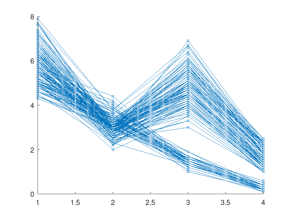
One line per flower through its four measurements

 plot (rm);

Example: 2

1. Lines coloured by group

 load fisheriris
 t = table (species, meas(:,1), meas(:,2), meas(:,3), meas(:,4), ...
            'VariableNames', {'species', 'meas1', 'meas2', 'meas3', 'meas4'});
 rm = fitrm (t, 'meas1-meas4 ~ species');

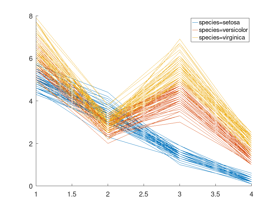
Group colours the lines by species, so a profile that one species follows and the others do not stands out

 plot (rm, 'Group', 'species', 'Marker', 'none');

RepeatedMeasuresModel: h = plotprofile (rm, X)

RepeatedMeasuresModel: h = plotprofile (rm, X, name, value)

plotprofile (rm, X) draws the estimated marginal means of margmean over the levels of the factor X, a categorical between-subject factor or a within-subject factor, and returns the line handles h. A numeric within-subject factor is drawn at its values; any other at the positions 1 to L of its L levels, labelled with them.

The name-value arguments are 'Group', the name of another factor, which draws one line per level of it and adds a legend; 'Marker', 'o' by default; and 'LineStyle', '-' by default.

See also: fitrm, RepeatedMeasuresModel.margmean, RepeatedMeasuresModel.plot

Example: 1

1. The marginal means of a between-subject factor

 load fisheriris
 t = table (species, meas(:,1), meas(:,2), meas(:,3), meas(:,4), ...
            'VariableNames', {'species', 'meas1', 'meas2', 'meas3', 'meas4'});
 rm = fitrm (t, 'meas1-meas4 ~ species');

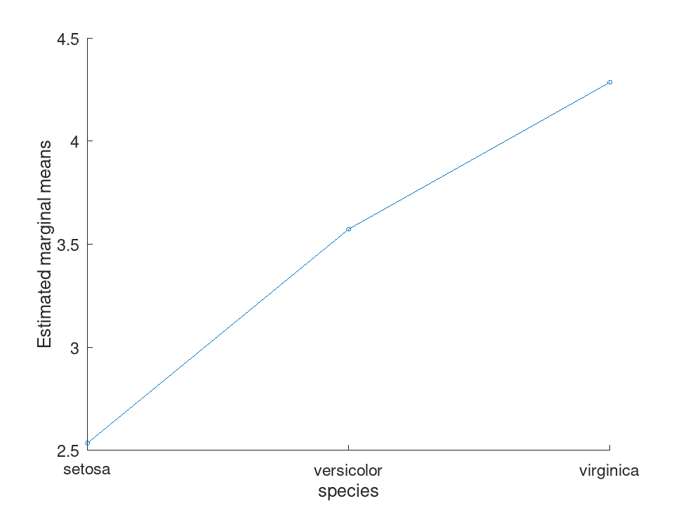
The mean over the four measurements, one point per species

 plotprofile (rm, 'species');

Example: 2

1. A profile over the measurements, one line per group

 load fisheriris
 t = table (species, meas(:,1), meas(:,2), meas(:,3), meas(:,4), ...
            'VariableNames', {'species', 'meas1', 'meas2', 'meas3', 'meas4'});
 Meas = table ([1, 2, 3, 4]', 'VariableNames', {'Measurements'});
 rm = fitrm (t, 'meas1-meas4 ~ species', 'WithinDesign', Meas);

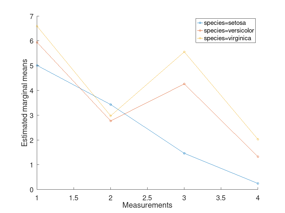
Lines that are not parallel are what ranova reports as the interaction of species with the measurements

 plotprofile (rm, 'Measurements', 'Group', 'species');